17  Dates and times

17.1 Introduction

This chapter will show you how to work with dates and times in R. At first glance, dates and times seem simple. You use them all the time in your regular life, and they don’t seem to cause much confusion. However, the more you learn about dates and times, the more complicated they seem to get!

To warm up think about how many days there are in a year, and how many hours there are in a day. You probably remembered that most years have 365 days, but leap years have 366. Do you know the full rule for determining if a year is a leap year¹? The number of hours in a day is a little less obvious: most days have 24 hours, but in places that use daylight saving time (DST), one day each year has 23 hours and another has 25.

Dates and times are hard because they have to reconcile two physical phenomena (the rotation of the Earth and its orbit around the sun) with a whole raft of geopolitical phenomena including months, time zones, and DST. This chapter won’t teach you every last detail about dates and times, but it will give you a solid grounding of practical skills that will help you with common data analysis challenges.

We’ll begin by showing you how to create date-times from various inputs, and then once you’ve got a date-time, how you can extract components like year, month, and day. We’ll then dive into the tricky topic of working with time spans, which come in a variety of flavors depending on what you’re trying to do. We’ll conclude with a brief discussion of the additional challenges posed by time zones.

17.1.1 Prerequisites

This chapter will focus on the lubridate package, which makes it easier to work with dates and times in R. As of the latest tidyverse release, lubridate is part of core tidyverse. We will also need nycflights13 for practice data.

library(tidyverse)
library(nycflights13)

17.2 Creating date/times

There are three types of date/time data that refer to an instant in time:

• A date. Tibbles print this as <date>.

• A time within a day. Tibbles print this as <time>.

• A date-time is a date plus a time: it uniquely identifies an instant in time (typically to the nearest second). Tibbles print this as <dttm>. Base R calls these POSIXct, but that doesn’t exactly trip off the tongue.

In this chapter we are going to focus on dates and date-times as R doesn’t have a native class for storing times. If you need one, you can use the hms package.

You should always use the simplest possible data type that works for your needs. That means if you can use a date instead of a date-time, you should. Date-times are substantially more complicated because of the need to handle time zones, which we’ll come back to at the end of the chapter.

To get the current date or date-time you can use today() or now():

today()
#> [1] "2024-12-25"
now()
#> [1] "2024-12-25 23:08:13 UTC"

Otherwise, the following sections describe the four ways you’re likely to create a date/time:

• While reading a file with readr.
• From a string.
• From individual date-time components.
• From an existing date/time object.

17.2.1 During import

If your CSV contains an ISO8601 date or date-time, you don’t need to do anything; readr will automatically recognize it:

csv <- "
  date,datetime
  2022-01-02,2022-01-02 05:12
"
read_csv(csv)
#> # A tibble: 1 × 2
#>   date       datetime           
#>   <date>     <dttm>             
#> 1 2022-01-02 2022-01-02 05:12:00

If you haven’t heard of ISO8601 before, it’s an international standard² for writing dates where the components of a date are organized from biggest to smallest separated by -. For example, in ISO8601 May 3 2022 is 2022-05-03. ISO8601 dates can also include times, where hour, minute, and second are separated by :, and the date and time components are separated by either a T or a space. For example, you could write 4:26pm on May 3 2022 as either 2022-05-03 16:26 or 2022-05-03T16:26.

For other date-time formats, you’ll need to use col_types plus col_date() or col_datetime() along with a date-time format. The date-time format used by readr is a standard used across many programming languages, describing a date component with a % followed by a single character. For example, %Y-%m-%d specifies a date that’s a year, -, month (as number) -, day. Table Table 17.1 lists all the options.

Table 17.1: All date formats understood by readr

Type	Code	Meaning	Example
Year	%Y	4 digit year	2021
	%y	2 digit year	21
Month	%m	Number	2
	%b	Abbreviated name	Feb
	%B	Full name	February
Day	%d	One or two digits	2
	%e	Two digits	02
Time	%H	24-hour hour	13
	%I	12-hour hour	1
	%p	AM/PM	pm
	%M	Minutes	35
	%S	Seconds	45
	%OS	Seconds with decimal component	45.35
	%Z	Time zone name	America/Chicago
	%z	Offset from UTC	+0800
Other	%.	Skip one non-digit	:
	%*	Skip any number of non-digits

And this code shows a few options applied to a very ambiguous date:

csv <- "
  date
  01/02/15
"

read_csv(csv, col_types = cols(date = col_date("%m/%d/%y")))
#> # A tibble: 1 × 1
#>   date      
#>   <date>    
#> 1 2015-01-02

read_csv(csv, col_types = cols(date = col_date("%d/%m/%y")))
#> # A tibble: 1 × 1
#>   date      
#>   <date>    
#> 1 2015-02-01

read_csv(csv, col_types = cols(date = col_date("%y/%m/%d")))
#> # A tibble: 1 × 1
#>   date      
#>   <date>    
#> 1 2001-02-15

Note that no matter how you specify the date format, it’s always displayed the same way once you get it into R.

If you’re using %b or %B and working with non-English dates, you’ll also need to provide a locale(). See the list of built-in languages in date_names_langs(), or create your own with date_names(),

17.2.2 From strings

The date-time specification language is powerful, but requires careful analysis of the date format. An alternative approach is to use lubridate’s helpers which attempt to automatically determine the format once you specify the order of the component. To use them, identify the order in which year, month, and day appear in your dates, then arrange “y”, “m”, and “d” in the same order. That gives you the name of the lubridate function that will parse your date. For example:

ymd("2017-01-31")
#> [1] "2017-01-31"
mdy("January 31st, 2017")
#> [1] "2017-01-31"
dmy("31-Jan-2017")
#> [1] "2017-01-31"

ymd() and friends create dates. To create a date-time, add an underscore and one or more of “h”, “m”, and “s” to the name of the parsing function:

ymd_hms("2017-01-31 20:11:59")
#> [1] "2017-01-31 20:11:59 UTC"
mdy_hm("01/31/2017 08:01")
#> [1] "2017-01-31 08:01:00 UTC"

You can also force the creation of a date-time from a date by supplying a timezone:

ymd("2017-01-31", tz = "UTC")
#> [1] "2017-01-31 UTC"

Here I use the UTC³ timezone which you might also know as GMT, or Greenwich Mean Time, the time at 0° longitude⁴ . It doesn’t use daylight saving time, making it a bit easier to compute with .

17.2.3 From individual components

Instead of a single string, sometimes you’ll have the individual components of the date-time spread across multiple columns. This is what we have in the flights data:

flights |> 
  select(year, month, day, hour, minute)
#> # A tibble: 336,776 × 5
#>    year month   day  hour minute
#>   <int> <int> <int> <dbl>  <dbl>
#> 1  2013     1     1     5     15
#> 2  2013     1     1     5     29
#> 3  2013     1     1     5     40
#> 4  2013     1     1     5     45
#> 5  2013     1     1     6      0
#> 6  2013     1     1     5     58
#> # ℹ 336,770 more rows

To create a date/time from this sort of input, use make_date() for dates, or make_datetime() for date-times:

flights |> 
  select(year, month, day, hour, minute) |> 
  mutate(departure = make_datetime(year, month, day, hour, minute))
#> # A tibble: 336,776 × 6
#>    year month   day  hour minute departure          
#>   <int> <int> <int> <dbl>  <dbl> <dttm>             
#> 1  2013     1     1     5     15 2013-01-01 05:15:00
#> 2  2013     1     1     5     29 2013-01-01 05:29:00
#> 3  2013     1     1     5     40 2013-01-01 05:40:00
#> 4  2013     1     1     5     45 2013-01-01 05:45:00
#> 5  2013     1     1     6      0 2013-01-01 06:00:00
#> 6  2013     1     1     5     58 2013-01-01 05:58:00
#> # ℹ 336,770 more rows

Let’s do the same thing for each of the four time columns in flights. The times are represented in a slightly odd format, so we use modulus arithmetic to pull out the hour and minute components. Once we’ve created the date-time variables, we focus in on the variables we’ll explore in the rest of the chapter.

make_datetime_100 <- function(year, month, day, time) {
  make_datetime(year, month, day, time %/% 100, time %% 100)
}

flights_dt <- flights |> 
  filter(!is.na(dep_time), !is.na(arr_time)) |> 
  mutate(
    dep_time = make_datetime_100(year, month, day, dep_time),
    arr_time = make_datetime_100(year, month, day, arr_time),
    sched_dep_time = make_datetime_100(year, month, day, sched_dep_time),
    sched_arr_time = make_datetime_100(year, month, day, sched_arr_time)
  ) |> 
  select(origin, dest, ends_with("delay"), ends_with("time"))

flights_dt
#> # A tibble: 328,063 × 9
#>   origin dest  dep_delay arr_delay dep_time            sched_dep_time     
#>   <chr>  <chr>     <dbl>     <dbl> <dttm>              <dttm>             
#> 1 EWR    IAH           2        11 2013-01-01 05:17:00 2013-01-01 05:15:00
#> 2 LGA    IAH           4        20 2013-01-01 05:33:00 2013-01-01 05:29:00
#> 3 JFK    MIA           2        33 2013-01-01 05:42:00 2013-01-01 05:40:00
#> 4 JFK    BQN          -1       -18 2013-01-01 05:44:00 2013-01-01 05:45:00
#> 5 LGA    ATL          -6       -25 2013-01-01 05:54:00 2013-01-01 06:00:00
#> 6 EWR    ORD          -4        12 2013-01-01 05:54:00 2013-01-01 05:58:00
#> # ℹ 328,057 more rows
#> # ℹ 3 more variables: arr_time <dttm>, sched_arr_time <dttm>, …

With this data, we can visualize the distribution of departure times across the year:

flights_dt |> 
  ggplot(aes(x = dep_time)) + 
  geom_freqpoly(binwidth = 86400) # 86400 seconds = 1 day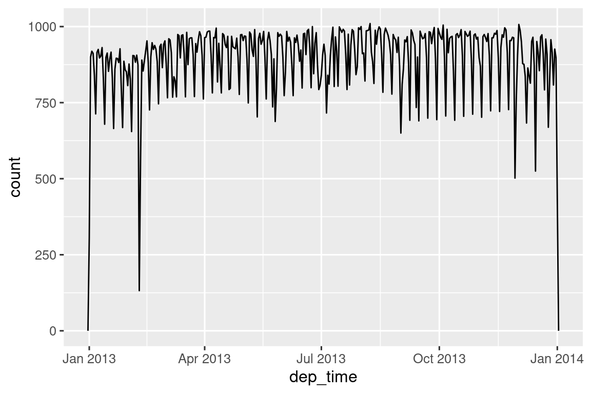

Or within a single day:

flights_dt |> 
  filter(dep_time < ymd(20130102)) |> 
  ggplot(aes(x = dep_time)) + 
  geom_freqpoly(binwidth = 600) # 600 s = 10 minutes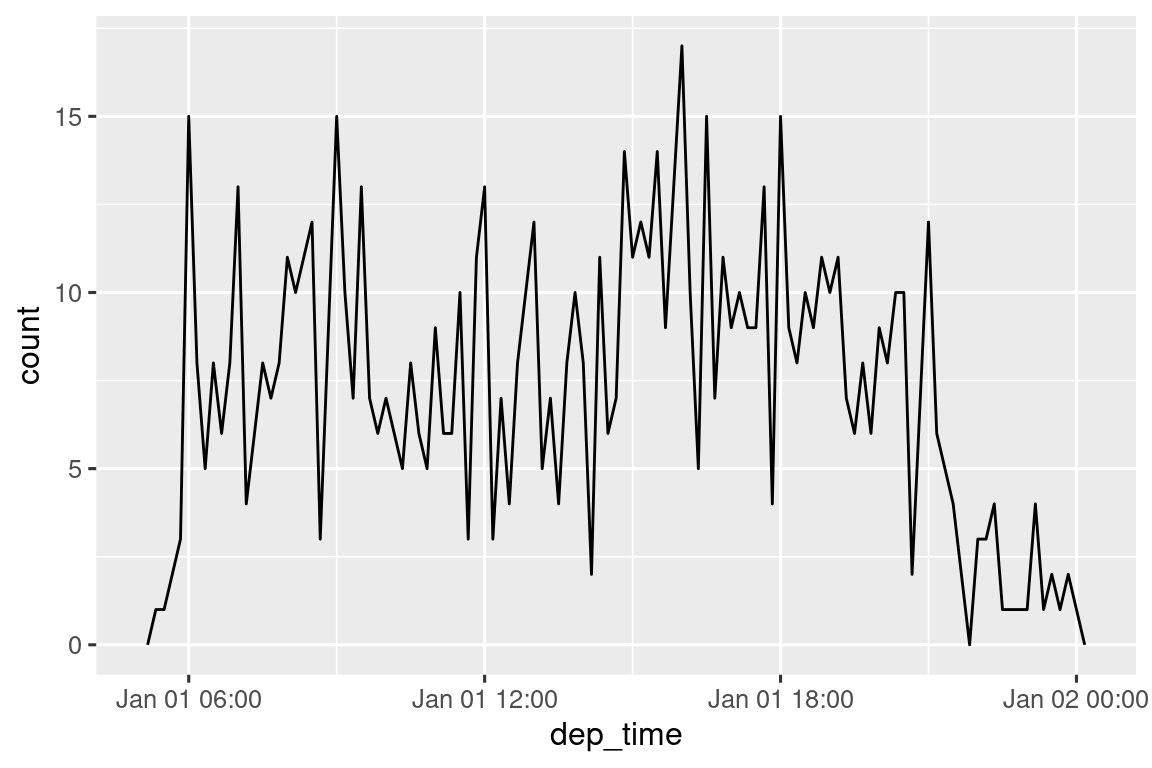

Note that when you use date-times in a numeric context (like in a histogram), 1 means 1 second, so a binwidth of 86400 means one day. For dates, 1 means 1 day.

17.2.4 From other types

You may want to switch between a date-time and a date. That’s the job of as_datetime() and as_date():

as_datetime(today())
#> [1] "2024-12-25 UTC"
as_date(now())
#> [1] "2024-12-25"

Sometimes you’ll get date/times as numeric offsets from the “Unix Epoch”, 1970-01-01. If the offset is in seconds, use as_datetime(); if it’s in days, use as_date().

as_datetime(60 * 60 * 10)
#> [1] "1970-01-01 10:00:00 UTC"
as_date(365 * 10 + 2)
#> [1] "1980-01-01"

17.2.5 Exercises

1. What happens if you parse a string that contains invalid dates?

   ymd(c("2010-10-10", "bananas"))

2. What does the tzone argument to today() do? Why is it important?

3. For each of the following date-times, show how you’d parse it using a readr column specification and a lubridate function.

   d1 <- "January 1, 2010"
   d2 <- "2015-Mar-07"
   d3 <- "06-Jun-2017"
   d4 <- c("August 19 (2015)", "July 1 (2015)")
   d5 <- "12/30/14" # Dec 30, 2014
   t1 <- "1705"
   t2 <- "11:15:10.12 PM"

17.3 Date-time components

Now that you know how to get date-time data into R’s date-time data structures, let’s explore what you can do with them. This section will focus on the accessor functions that let you get and set individual components. The next section will look at how arithmetic works with date-times.

17.3.1 Getting components

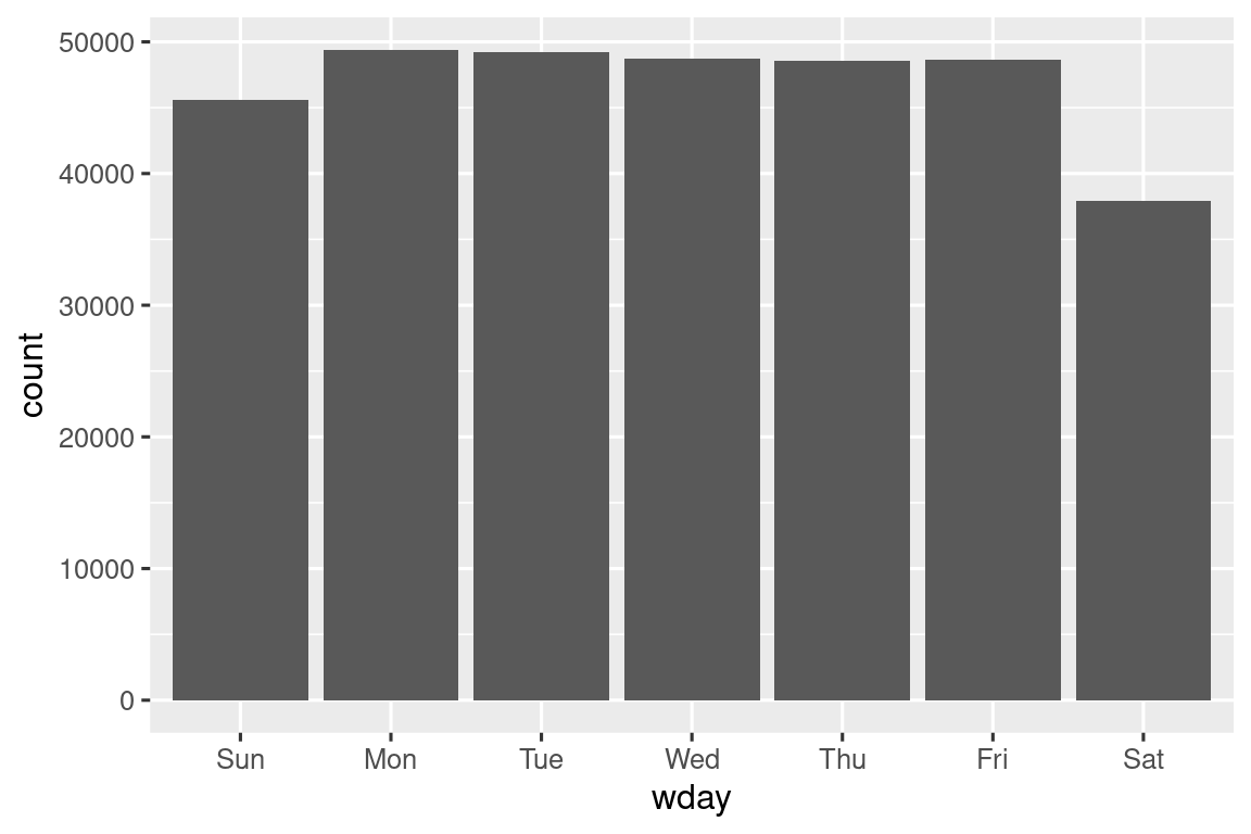
You can pull out individual parts of the date with the accessor functions year(), month(), mday() (day of the month), yday() (day of the year), wday() (day of the week), hour(), minute(), and second(). These are effectively the opposites of make_datetime().

datetime <- ymd_hms("2026-07-08 12:34:56")

year(datetime)
#> [1] 2026
month(datetime)
#> [1] 7
mday(datetime)
#> [1] 8

yday(datetime)
#> [1] 189
wday(datetime)
#> [1] 4

For month() and wday() you can set label = TRUE to return the abbreviated name of the month or day of the week. Set abbr = FALSE to return the full name.

month(datetime, label = TRUE)
#> [1] Jul
#> 12 Levels: Jan < Feb < Mar < Apr < May < Jun < Jul < Aug < Sep < ... < Dec
wday(datetime, label = TRUE, abbr = FALSE)
#> [1] Wednesday
#> 7 Levels: Sunday < Monday < Tuesday < Wednesday < Thursday < ... < Saturday

We can use wday() to see that more flights depart during the week than on the weekend:

flights_dt |> 
  mutate(wday = wday(dep_time, label = TRUE)) |> 
  ggplot(aes(x = wday)) +
  geom_bar()

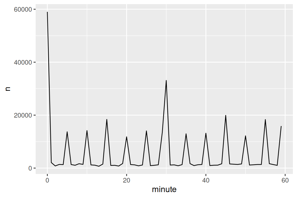
We can also look at the average departure delay by minute within the hour. There’s an interesting pattern: flights leaving in minutes 20-30 and 50-60 have much lower delays than the rest of the hour!

flights_dt |> 
  mutate(minute = minute(dep_time)) |> 
  group_by(minute) |> 
  summarize(
    avg_delay = mean(dep_delay, na.rm = TRUE),
    n = n()
  ) |> 
  ggplot(aes(x = minute, y = avg_delay)) +
  geom_line()

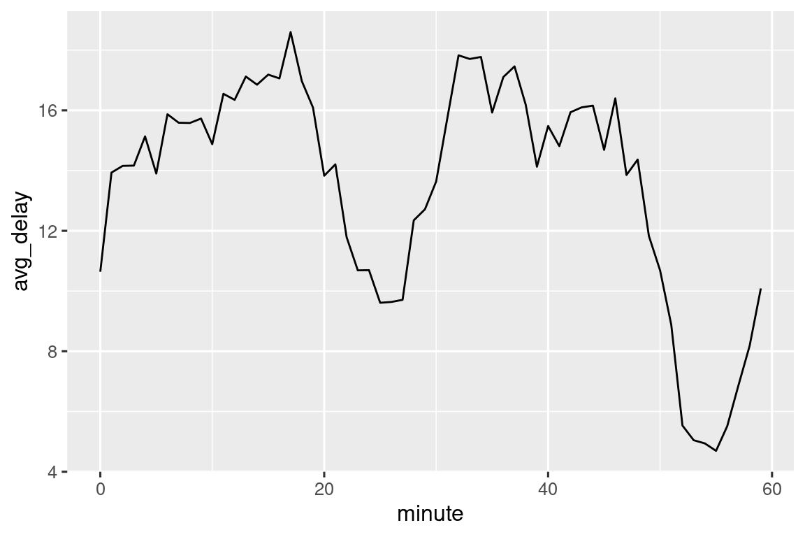
Interestingly, if we look at the scheduled departure time we don’t see such a strong pattern:

sched_dep <- flights_dt |> 
  mutate(minute = minute(sched_dep_time)) |> 
  group_by(minute) |> 
  summarize(
    avg_delay = mean(arr_delay, na.rm = TRUE),
    n = n()
  )

ggplot(sched_dep, aes(x = minute, y = avg_delay)) +
  geom_line()

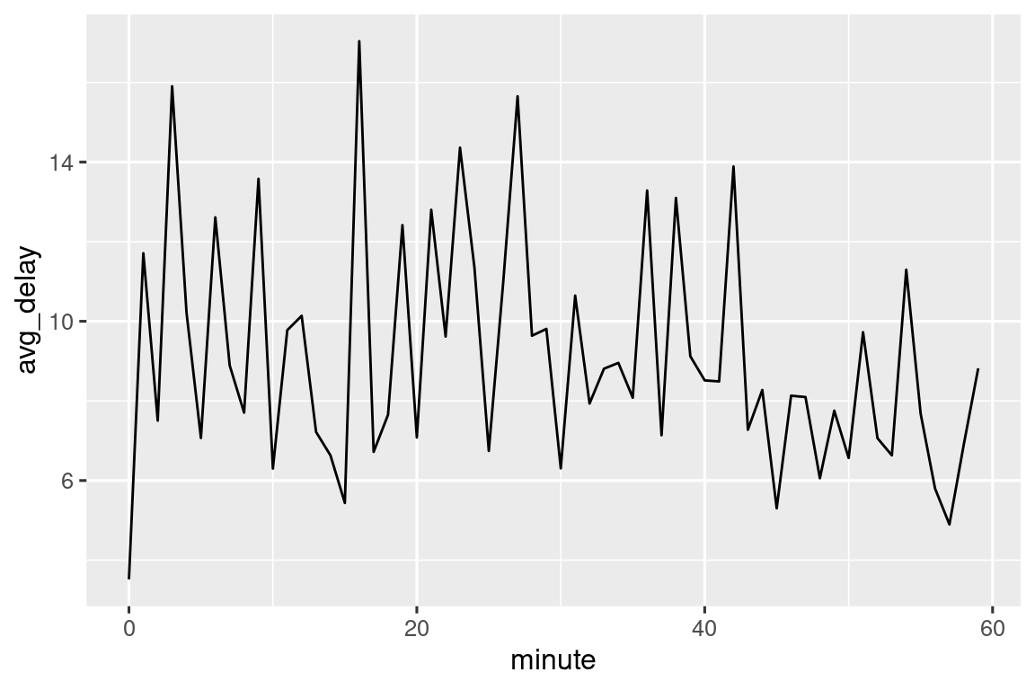
So why do we see that pattern with the actual departure times? Well, like much data collected by humans, there’s a strong bias towards flights leaving at “nice” departure times, as Figure 17.1 shows. Always be alert for this sort of pattern whenever you work with data that involves human judgement!

Figure 17.1: A frequency polygon showing the number of flights scheduled to depart each hour. You can see a strong preference for round numbers like 0 and 30 and generally for numbers that are a multiple of five.

17.3.2 Rounding

An alternative approach to plotting individual components is to round the date to a nearby unit of time, with floor_date(), round_date(), and ceiling_date(). Each function takes a vector of dates to adjust and then the name of the unit to round down (floor), round up (ceiling), or round to. This, for example, allows us to plot the number of flights per week:

flights_dt |> 
  count(week = floor_date(dep_time, "week")) |> 
  ggplot(aes(x = week, y = n)) +
  geom_line() + 
  geom_point()

You can use rounding to show the distribution of flights across the course of a day by computing the difference between dep_time and the earliest instant of that day:

flights_dt |> 
  mutate(dep_hour = dep_time - floor_date(dep_time, "day")) |> 
  ggplot(aes(x = dep_hour)) +
  geom_freqpoly(binwidth = 60 * 30)
#> Don't know how to automatically pick scale for object of type <difftime>.
#> Defaulting to continuous.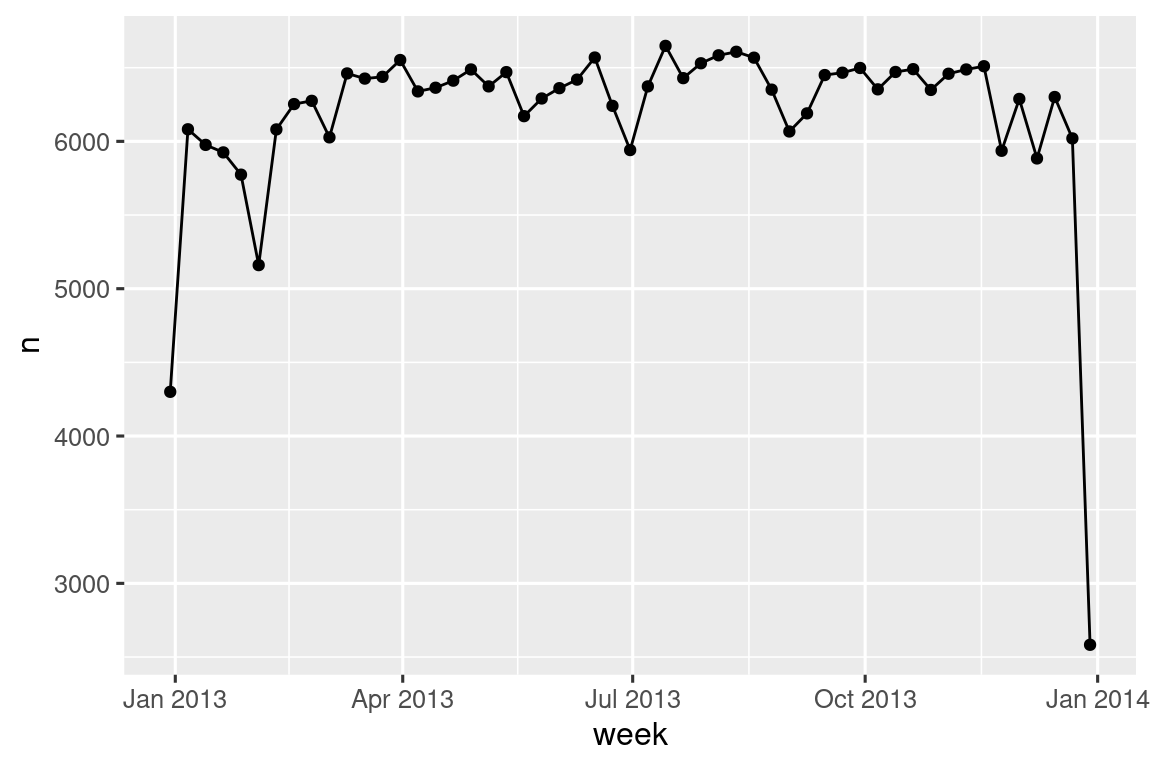

Computing the difference between a pair of date-times yields a difftime (more on that in Section 17.4.3). We can convert that to an hms object to get a more useful x-axis:

flights_dt |> 
  mutate(dep_hour = hms::as_hms(dep_time - floor_date(dep_time, "day"))) |> 
  ggplot(aes(x = dep_hour)) +
  geom_freqpoly(binwidth = 60 * 30)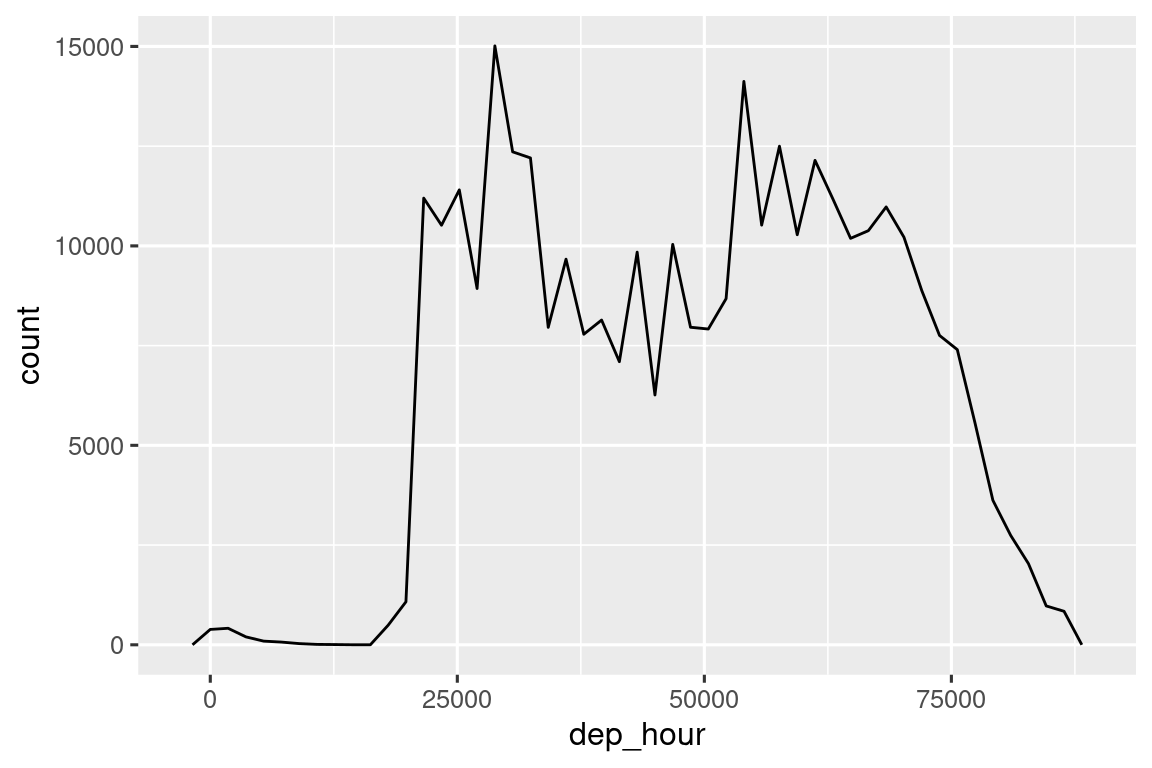

17.3.3 Modifying components

You can also use each accessor function to modify the components of a date/time. This doesn’t come up much in data analysis, but can be useful when cleaning data that has clearly incorrect dates.

(datetime <- ymd_hms("2026-07-08 12:34:56"))
#> [1] "2026-07-08 12:34:56 UTC"

year(datetime) <- 2030
datetime
#> [1] "2030-07-08 12:34:56 UTC"
month(datetime) <- 01
datetime
#> [1] "2030-01-08 12:34:56 UTC"
hour(datetime) <- hour(datetime) + 1
datetime
#> [1] "2030-01-08 13:34:56 UTC"

Alternatively, rather than modifying an existing variable, you can create a new date-time with update(). This also allows you to set multiple values in one step:

update(datetime, year = 2030, month = 2, mday = 2, hour = 2)
#> [1] "2030-02-02 02:34:56 UTC"

If values are too big, they will roll-over:

update(ymd("2023-02-01"), mday = 30)
#> [1] "2023-03-02"
update(ymd("2023-02-01"), hour = 400)
#> [1] "2023-02-17 16:00:00 UTC"

17.3.4 Exercises

1. How does the distribution of flight times within a day change over the course of the year?

2. Compare dep_time, sched_dep_time and dep_delay. Are they consistent? Explain your findings.

3. Compare air_time with the duration between the departure and arrival. Explain your findings. (Hint: consider the location of the airport.)

4. How does the average delay time change over the course of a day? Should you use dep_time or sched_dep_time? Why?

5. On what day of the week should you leave if you want to minimise the chance of a delay?

6. What makes the distribution of diamonds$carat and flights$sched_dep_time similar?

7. Confirm our hypothesis that the early departures of flights in minutes 20-30 and 50-60 are caused by scheduled flights that leave early. Hint: create a binary variable that tells you whether or not a flight was delayed.

17.4 Time spans

Next you’ll learn about how arithmetic with dates works, including subtraction, addition, and division. Along the way, you’ll learn about three important classes that represent time spans:

• Durations, which represent an exact number of seconds.
• Periods, which represent human units like weeks and months.
• Intervals, which represent a starting and ending point.

How do you pick between duration, periods, and intervals? As always, pick the simplest data structure that solves your problem. If you only care about physical time, use a duration; if you need to add human times, use a period; if you need to figure out how long a span is in human units, use an interval.

17.4.1 Durations

In R, when you subtract two dates, you get a difftime object:

# How old is Hadley?
h_age <- today() - ymd("1979-10-14")
h_age
#> Time difference of 16509 days

A difftime class object records a time span of seconds, minutes, hours, days, or weeks. This ambiguity can make difftimes a little painful to work with, so lubridate provides an alternative which always uses seconds: the duration.

as.duration(h_age)
#> [1] "1426377600s (~45.2 years)"

Durations come with a bunch of convenient constructors:

dseconds(15)
#> [1] "15s"
dminutes(10)
#> [1] "600s (~10 minutes)"
dhours(c(12, 24))
#> [1] "43200s (~12 hours)" "86400s (~1 days)"
ddays(0:5)
#> [1] "0s"                "86400s (~1 days)"  "172800s (~2 days)"
#> [4] "259200s (~3 days)" "345600s (~4 days)" "432000s (~5 days)"
dweeks(3)
#> [1] "1814400s (~3 weeks)"
dyears(1)
#> [1] "31557600s (~1 years)"

Durations always record the time span in seconds. Larger units are created by converting minutes, hours, days, weeks, and years to seconds: 60 seconds in a minute, 60 minutes in an hour, 24 hours in a day, and 7 days in a week. Larger time units are more problematic. A year uses the “average” number of days in a year, i.e. 365.25. There’s no way to convert a month to a duration, because there’s just too much variation.

You can add and multiply durations:

2 * dyears(1)
#> [1] "63115200s (~2 years)"
dyears(1) + dweeks(12) + dhours(15)
#> [1] "38869200s (~1.23 years)"

You can add and subtract durations to and from days:

tomorrow <- today() + ddays(1)
last_year <- today() - dyears(1)

However, because durations represent an exact number of seconds, sometimes you might get an unexpected result:

one_am <- ymd_hms("2026-03-08 01:00:00", tz = "America/New_York")

one_am
#> [1] "2026-03-08 01:00:00 EST"
one_am + ddays(1)
#> [1] "2026-03-09 02:00:00 EDT"

Why is one day after 1am March 8, 2am March 9? If you look carefully at the date you might also notice that the time zones have changed. March 8 only has 23 hours because it’s when DST starts, so if we add a full days worth of seconds we end up with a different time.

17.4.2 Periods

To solve this problem, lubridate provides periods. Periods are time spans but don’t have a fixed length in seconds, instead they work with “human” times, like days and months. That allows them to work in a more intuitive way:

one_am
#> [1] "2026-03-08 01:00:00 EST"
one_am + days(1)
#> [1] "2026-03-09 01:00:00 EDT"

Like durations, periods can be created with a number of friendly constructor functions.

hours(c(12, 24))
#> [1] "12H 0M 0S" "24H 0M 0S"
days(7)
#> [1] "7d 0H 0M 0S"
months(1:6)
#> [1] "1m 0d 0H 0M 0S" "2m 0d 0H 0M 0S" "3m 0d 0H 0M 0S" "4m 0d 0H 0M 0S"
#> [5] "5m 0d 0H 0M 0S" "6m 0d 0H 0M 0S"

You can add and multiply periods:

10 * (months(6) + days(1))
#> [1] "60m 10d 0H 0M 0S"
days(50) + hours(25) + minutes(2)
#> [1] "50d 25H 2M 0S"

And of course, add them to dates. Compared to durations, periods are more likely to do what you expect:

# A leap year
ymd("2024-01-01") + dyears(1)
#> [1] "2024-12-31 06:00:00 UTC"
ymd("2024-01-01") + years(1)
#> [1] "2025-01-01"

# Daylight saving time
one_am + ddays(1)
#> [1] "2026-03-09 02:00:00 EDT"
one_am + days(1)
#> [1] "2026-03-09 01:00:00 EDT"

Let’s use periods to fix an oddity related to our flight dates. Some planes appear to have arrived at their destination before they departed from New York City.

flights_dt |> 
  filter(arr_time < dep_time) 
#> # A tibble: 10,633 × 9
#>   origin dest  dep_delay arr_delay dep_time            sched_dep_time     
#>   <chr>  <chr>     <dbl>     <dbl> <dttm>              <dttm>             
#> 1 EWR    BQN           9        -4 2013-01-01 19:29:00 2013-01-01 19:20:00
#> 2 JFK    DFW          59        NA 2013-01-01 19:39:00 2013-01-01 18:40:00
#> 3 EWR    TPA          -2         9 2013-01-01 20:58:00 2013-01-01 21:00:00
#> 4 EWR    SJU          -6       -12 2013-01-01 21:02:00 2013-01-01 21:08:00
#> 5 EWR    SFO          11       -14 2013-01-01 21:08:00 2013-01-01 20:57:00
#> 6 LGA    FLL         -10        -2 2013-01-01 21:20:00 2013-01-01 21:30:00
#> # ℹ 10,627 more rows
#> # ℹ 3 more variables: arr_time <dttm>, sched_arr_time <dttm>, …

These are overnight flights. We used the same date information for both the departure and the arrival times, but these flights arrived on the following day. We can fix this by adding days(1) to the arrival time of each overnight flight.

flights_dt <- flights_dt |> 
  mutate(
    overnight = arr_time < dep_time,
    arr_time = arr_time + days(overnight),
    sched_arr_time = sched_arr_time + days(overnight)
  )

Now all of our flights obey the laws of physics.

flights_dt |> 
  filter(arr_time < dep_time) 
#> # A tibble: 0 × 10
#> # ℹ 10 variables: origin <chr>, dest <chr>, dep_delay <dbl>,
#> #   arr_delay <dbl>, dep_time <dttm>, sched_dep_time <dttm>, …

17.4.3 Intervals

What does dyears(1) / ddays(365) return? It’s not quite one, because dyears() is defined as the number of seconds per average year, which is 365.25 days.

What does years(1) / days(1) return? Well, if the year was 2015 it should return 365, but if it was 2016, it should return 366! There’s not quite enough information for lubridate to give a single clear answer. What it does instead is give an estimate:

years(1) / days(1)
#> [1] 365.25

If you want a more accurate measurement, you’ll have to use an interval. An interval is a pair of starting and ending date times, or you can think of it as a duration with a starting point.

You can create an interval by writing start %--% end:

y2023 <- ymd("2023-01-01") %--% ymd("2024-01-01")
y2024 <- ymd("2024-01-01") %--% ymd("2025-01-01")

y2023
#> [1] 2023-01-01 UTC--2024-01-01 UTC
y2024
#> [1] 2024-01-01 UTC--2025-01-01 UTC

You could then divide it by days() to find out how many days fit in the year:

y2023 / days(1)
#> [1] 365
y2024 / days(1)
#> [1] 366

17.4.4 Exercises

1. Explain days(!overnight) and days(overnight) to someone who has just started learning R. What is the key fact you need to know?

2. Create a vector of dates giving the first day of every month in 2015. Create a vector of dates giving the first day of every month in the current year.

3. Write a function that given your birthday (as a date), returns how old you are in years.

4. Why can’t (today() %--% (today() + years(1))) / months(1) work?

17.5 Time zones

Time zones are an enormously complicated topic because of their interaction with geopolitical entities. Fortunately we don’t need to dig into all the details as they’re not all important for data analysis, but there are a few challenges we’ll need to tackle head on.

The first challenge is that everyday names of time zones tend to be ambiguous. For example, if you’re American you’re probably familiar with EST, or Eastern Standard Time. However, both Australia and Canada also have EST! To avoid confusion, R uses the international standard IANA time zones. These use a consistent naming scheme {area}/{location}, typically in the form {continent}/{city} or {ocean}/{city}. Examples include “America/New_York”, “Europe/Paris”, and “Pacific/Auckland”.

You might wonder why the time zone uses a city, when typically you think of time zones as associated with a country or region within a country. This is because the IANA database has to record decades worth of time zone rules. Over the course of decades, countries change names (or break apart) fairly frequently, but city names tend to stay the same. Another problem is that the name needs to reflect not only the current behavior, but also the complete history. For example, there are time zones for both “America/New_York” and “America/Detroit”. These cities both currently use Eastern Standard Time but in 1969-1972 Michigan (the state in which Detroit is located), did not follow DST, so it needs a different name. It’s worth reading the raw time zone database (available at https://www.iana.org/time-zones) just to read some of these stories!

You can find out what R thinks your current time zone is with Sys.timezone():

Sys.timezone()
#> [1] "UTC"

(If R doesn’t know, you’ll get an NA.)

And see the complete list of all time zone names with OlsonNames():

length(OlsonNames())
#> [1] 597
head(OlsonNames())
#> [1] "Africa/Abidjan"     "Africa/Accra"       "Africa/Addis_Ababa"
#> [4] "Africa/Algiers"     "Africa/Asmara"      "Africa/Asmera"

In R, the time zone is an attribute of the date-time that only controls printing. For example, these three objects represent the same instant in time:

x1 <- ymd_hms("2024-06-01 12:00:00", tz = "America/New_York")
x1
#> [1] "2024-06-01 12:00:00 EDT"

x2 <- ymd_hms("2024-06-01 18:00:00", tz = "Europe/Copenhagen")
x2
#> [1] "2024-06-01 18:00:00 CEST"

x3 <- ymd_hms("2024-06-02 04:00:00", tz = "Pacific/Auckland")
x3
#> [1] "2024-06-02 04:00:00 NZST"

You can verify that they’re the same time using subtraction:

x1 - x2
#> Time difference of 0 secs
x1 - x3
#> Time difference of 0 secs

Unless otherwise specified, lubridate always uses UTC. UTC (Coordinated Universal Time) is the standard time zone used by the scientific community and is roughly equivalent to GMT (Greenwich Mean Time). It does not have DST, which makes a convenient representation for computation. Operations that combine date-times, like c(), will often drop the time zone. In that case, the date-times will display in the time zone of the first element:

x4 <- c(x1, x2, x3)
x4
#> [1] "2024-06-01 12:00:00 EDT" "2024-06-01 12:00:00 EDT"
#> [3] "2024-06-01 12:00:00 EDT"

You can change the time zone in two ways:

• Keep the instant in time the same, and change how it’s displayed. Use this when the instant is correct, but you want a more natural display.

  x4a <- with_tz(x4, tzone = "Australia/Lord_Howe")
  x4a
  #> [1] "2024-06-02 02:30:00 +1030" "2024-06-02 02:30:00 +1030"
  #> [3] "2024-06-02 02:30:00 +1030"
  x4a - x4
  #> Time differences in secs
  #> [1] 0 0 0

  (This also illustrates another challenge of times zones: they’re not all integer hour offsets!)

• Change the underlying instant in time. Use this when you have an instant that has been labelled with the incorrect time zone, and you need to fix it.

  x4b <- force_tz(x4, tzone = "Australia/Lord_Howe")
  x4b
  #> [1] "2024-06-01 12:00:00 +1030" "2024-06-01 12:00:00 +1030"
  #> [3] "2024-06-01 12:00:00 +1030"
  x4b - x4
  #> Time differences in hours
  #> [1] -14.5 -14.5 -14.5

17.6 Summary

This chapter has introduced you to the tools that lubridate provides to help you work with date-time data. Working with dates and times can seem harder than necessary, but hopefully this chapter has helped you see why — date-times are more complex than they seem at first glance, and handling every possible situation adds complexity. Even if your data never crosses a day light savings boundary or involves a leap year, the functions need to be able to handle it.

The next chapter gives a round up of missing values. You’ve seen them in a few places and have no doubt encounter in your own analysis, and it’s now time to provide a grab bag of useful techniques for dealing with them.

---

1. A year is a leap year if it’s divisible by 4, unless it’s also divisible by 100, except if it’s also divisible by 400. In other words, in every set of 400 years, there’s 97 leap years.

2. https://xkcd.com/1179/

3. You might wonder what UTC stands for. It’s a compromise between the English “Coordinated Universal Time” and French “Temps Universel Coordonné”.

4. No prizes for guessing which country came up with the longitude system.