25 Functions
25.1 Introduction
One of the best ways to improve your reach as a data scientist is to write functions. Functions allow you to automate common tasks in a more powerful and general way than copy-and-pasting. Writing a function has four big advantages over using copy-and-paste:
You can give a function an evocative name that makes your code easier to understand.
As requirements change, you only need to update code in one place, instead of many.
You eliminate the chance of making incidental mistakes when you copy and paste (i.e. updating a variable name in one place, but not in another).
It makes it easier to reuse work from project-to-project, increasing your productivity over time.
A good rule of thumb is to consider writing a function whenever you’ve copied and pasted a block of code more than twice (i.e. you now have three copies of the same code). In this chapter, you’ll learn about three useful types of functions:
- Vector functions take one or more vectors as input and return a vector as output.
- Data frame functions take a data frame as input and return a data frame as output.
- Plot functions that take a data frame as input and return a plot as output.
Each of these sections includes many examples to help you generalize the patterns that you see. These examples wouldn’t be possible without the help of folks of twitter, and we encourage you to follow the links in the comments to see the original inspirations. You might also want to read the original motivating tweets for general functions and plotting functions to see even more functions.
25.1.1 Prerequisites
We’ll wrap up a variety of functions from around the tidyverse. We’ll also use nycflights13 as a source of familiar data to use our functions with.
25.2 Vector functions
We’ll begin with vector functions: functions that take one or more vectors and return a vector result. For example, take a look at this code. What does it do?
df <- tibble(
  a = rnorm(5),
  b = rnorm(5),
  c = rnorm(5),
  d = rnorm(5),
)

df |> mutate(
  a = (a - min(a, na.rm = TRUE)) /
    (max(a, na.rm = TRUE) - min(a, na.rm = TRUE)),
  b = (b - min(a, na.rm = TRUE)) /
    (max(b, na.rm = TRUE) - min(b, na.rm = TRUE)),
  c = (c - min(c, na.rm = TRUE)) /
    (max(c, na.rm = TRUE) - min(c, na.rm = TRUE)),
  d = (d - min(d, na.rm = TRUE)) /
    (max(d, na.rm = TRUE) - min(d, na.rm = TRUE)),
)
#> # A tibble: 5 × 4
#>       a       b     c     d
#>   <dbl>   <dbl> <dbl> <dbl>
#> 1 0.339  0.387  0.291 0
#> 2 0.880 -0.613  0.611 0.557
#> 3 0     -0.0833 1     0.752
#> 4 0.795 -0.0822 0     1
#> 5 1     -0.0952 0.580 0.394
You might be able to puzzle out that this rescales each column to have a range from 0 to 1. But did you spot the mistake? When Hadley wrote this code he made an error when copying-and-pasting and forgot to change an a to a b. Preventing this type of mistake is one very good reason to learn how to write functions.
25.2.1 Writing a function
To write a function you need to first analyse your repeated code to figure what parts are constant and what parts vary. If we take the code above and pull it outside of mutate(), it’s a little easier to see the pattern because each repetition is now one line:
To make this a bit clearer we can replace the bit that varies with █:
(█ - min(█, na.rm = TRUE)) / (max(█, na.rm = TRUE) - min(█, na.rm = TRUE))To turn this into a function you need three things:
A name. Here we’ll use
rescale01because this function rescales a vector to lie between 0 and 1.The arguments. The arguments are things that vary across calls and our analysis above tells us that we have just one. We’ll call it
xbecause this is the conventional name for a numeric vector.The body. The body is the code that’s repeated across all the calls.
Then you create a function by following the template:
name <- function(arguments) {
  body
}
For this case that leads to:
At this point you might test with a few simple inputs to make sure you’ve captured the logic correctly:
Then you can rewrite the call to mutate() as:
df |> mutate(
  a = rescale01(a),
  b = rescale01(b),
  c = rescale01(c),
  d = rescale01(d),
)
#> # A tibble: 5 × 4
#>       a     b     c     d
#>   <dbl> <dbl> <dbl> <dbl>
#> 1 0.339 1     0.291 0
#> 2 0.880 0     0.611 0.557
#> 3 0     0.530 1     0.752
#> 4 0.795 0.531 0     1
#> 5 1     0.518 0.580 0.394
(In Chapter 26, you’ll learn how to use across() to reduce the duplication even further so all you need is df |> mutate(across(a:d, rescale01))).
25.2.2 Improving our function
You might notice that the rescale01() function does some unnecessary work — instead of computing min() twice and max() once we could instead compute both the minimum and maximum in one step with range():
rescale01 <- function(x) {
  rng <- range(x, na.rm = TRUE)
  (x - rng[1]) / (rng[2] - rng[1])
}
Or you might try this function on a vector that includes an infinite value:
x <- c(1:10, Inf)
rescale01(x)
#>  [1]   0   0   0   0   0   0   0   0   0   0 NaN
That result is not particularly useful so we could ask range() to ignore infinite values:
rescale01 <- function(x) {
  rng <- range(x, na.rm = TRUE, finite = TRUE)
  (x - rng[1]) / (rng[2] - rng[1])
}

rescale01(x)
#>  [1] 0.0000000 0.1111111 0.2222222 0.3333333 0.4444444 0.5555556 0.6666667
#>  [8] 0.7777778 0.8888889 1.0000000       Inf
These changes illustrate an important benefit of functions: because we’ve moved the repeated code into a function, we only need to make the change in one place.
25.2.3 Mutate functions
Now that you’ve got the basic idea of functions, let’s take a look at a whole bunch of examples. We’ll start by looking at “mutate” functions, i.e. functions that work well inside of mutate() and filter() because they return an output of the same length as the input.
Let’s start with a simple variation of rescale01(). Maybe you want to compute the Z-score, rescaling a vector to have a mean of zero and a standard deviation of one:
Or maybe you want to wrap up a straightforward case_when() and give it a useful name. For example, this clamp() function ensures all values of a vector lie in between a minimum or a maximum:
clamp <- function(x, min, max) {
  case_when(
    x < min ~ min,
    x > max ~ max,
    .default = x
  )
}

clamp(1:10, min = 3, max = 7)
#>  [1] 3 3 3 4 5 6 7 7 7 7
Of course functions don’t just need to work with numeric variables. You might want to do some repeated string manipulation. Maybe you need to make the first character uppercase:
first_upper <- function(x) {
  str_sub(x, 1, 1) <- str_to_upper(str_sub(x, 1, 1))
  x
}

first_upper("hello")
#> [1] "Hello"
Or maybe you want to strip percent signs, commas, and dollar signs from a string before converting it into a number:
# https://twitter.com/NVlabormarket/status/1571939851922198530
clean_number <- function(x) {
  is_pct <- str_detect(x, "%")
  num <- x |>
    str_remove_all("%") |>
    str_remove_all(",") |>
    str_remove_all(fixed("$")) |>
    as.numeric()
  if_else(is_pct, num / 100, num)
}

clean_number("$12,300")
#> [1] 12300
clean_number("45%")
#> [1] 0.45
Sometimes your functions will be highly specialized for one data analysis step. For example, if you have a bunch of variables that record missing values as 997, 998, or 999, you might want to write a function to replace them with NA:
We’ve focused on examples that take a single vector because we think they’re the most common. But there’s no reason that your function can’t take multiple vector inputs.
25.2.4 Summary functions
Another important family of vector functions is summary functions, functions that return a single value for use in summarize(). Sometimes this can just be a matter of setting a default argument or two:
commas <- function(x) {
  str_flatten(x, collapse = ", ", last = " and ")
}

commas(c("cat", "dog", "pigeon"))
#> [1] "cat, dog and pigeon"
Or you might wrap up a simple computation, like for the coefficient of variation, which divides the standard deviation by the mean:
Or maybe you just want to make a common pattern easier to remember by giving it a memorable name:
You can also write functions with multiple vector inputs. For example, maybe you want to compute the mean absolute percentage error to help you compare model predictions with actual values:
Once you start writing functions, there are two RStudio shortcuts that are super useful:
To find the definition of a function that you’ve written, place the cursor on the name of the function and press
F2.To quickly jump to a function, press
Ctrl + .to open the fuzzy file and function finder and type the first few letters of your function name. You can also navigate to files, Quarto sections, and more, making it a very handy navigation tool.
25.2.5 Exercises
-
Practice turning the following code snippets into functions. Think about what each function does. What would you call it? How many arguments does it need?
In the second variant of
rescale01(), infinite values are left unchanged. Can you rewriterescale01()so that-Infis mapped to 0, andInfis mapped to 1?Given a vector of birthdates, write a function to compute the age in years.
Write your own functions to compute the variance and skewness of a numeric vector. You can look up the definitions on Wikipedia or elsewhere.
Write
both_na(), a summary function that takes two vectors of the same length and returns the number of positions that have anNAin both vectors.-
Read the documentation to figure out what the following functions do. Why are they useful even though they are so short?
is_directory <- function(x) {
  file.info(x)$isdir
}
is_readable <- function(x) {
  file.access(x, 4) == 0
}
25.3 Data frame functions
Vector functions are useful for pulling out code that’s repeated within a dplyr verb. But you’ll often also repeat the verbs themselves, particularly within a large pipeline. When you notice yourself copying and pasting multiple verbs multiple times, you might think about writing a data frame function. Data frame functions work like dplyr verbs: they take a data frame as the first argument, some extra arguments that say what to do with it, and return a data frame or a vector.
To let you write a function that uses dplyr verbs, we’ll first introduce you to the challenge of indirection and how you can overcome it with embracing, {{ }}. With this theory under your belt, we’ll then show you a bunch of examples to illustrate what you might do with it.
25.3.1 Indirection and tidy evaluation
When you start writing functions that use dplyr verbs you rapidly hit the problem of indirection. Let’s illustrate the problem with a very simple function: grouped_mean(). The goal of this function is to compute the mean of mean_var grouped by group_var:
If we try and use it, we get an error:
diamonds |> grouped_mean(cut, carat)
#> Error in `group_by()`:
#> ! Must group by variables found in `.data`.
#> ✖ Column `group_var` is not found.
To make the problem a bit more clear, we can use a made up data frame:
df <- tibble(
  mean_var = 1,
  group_var = "g",
  group = 1,
  x = 10,
  y = 100
)

df |> grouped_mean(group, x)
#> # A tibble: 1 × 2
#>   group_var `mean(mean_var)`
#>   <chr>                <dbl>
#> 1 g                        1
df |> grouped_mean(group, y)
#> # A tibble: 1 × 2
#>   group_var `mean(mean_var)`
#>   <chr>                <dbl>
#> 1 g                        1
Regardless of how we call grouped_mean() it always does df |> group_by(group_var) |> summarize(mean(mean_var)), instead of df |> group_by(group) |> summarize(mean(x)) or df |> group_by(group) |> summarize(mean(y)). This is a problem of indirection, and it arises because dplyr uses tidy evaluation to allow you to refer to the names of variables inside your data frame without any special treatment.
Tidy evaluation is great 95% of the time because it makes your data analyses very concise as you never have to say which data frame a variable comes from; it’s obvious from the context. The downside of tidy evaluation comes when we want to wrap up repeated tidyverse code into a function. Here we need some way to tell group_by() and summarize() not to treat group_var and mean_var as the name of the variables, but instead look inside them for the variable we actually want to use.
Tidy evaluation includes a solution to this problem called embracing 🤗. Embracing a variable means to wrap it in braces so (e.g.) var becomes {{ var }}. Embracing a variable tells dplyr to use the value stored inside the argument, not the argument as the literal variable name. One way to remember what’s happening is to think of {{ }} as looking down a tunnel — {{ var }} will make a dplyr function look inside of var rather than looking for a variable called var.
So to make grouped_mean() work, we need to surround group_var and mean_var with {{ }}:
Success!
25.3.2 When to embrace?
So the key challenge in writing data frame functions is figuring out which arguments need to be embraced. Fortunately, this is easy because you can look it up from the documentation 😄. There are two terms to look for in the docs which correspond to the two most common sub-types of tidy evaluation:
Data-masking: this is used in functions like
arrange(),filter(), andsummarize()that compute with variables.Tidy-selection: this is used for functions like
select(),relocate(), andrename()that select variables.
Your intuition about which arguments use tidy evaluation should be good for many common functions — just think about whether you can compute (e.g., x + 1) or select (e.g., a:x).
In the following sections, we’ll explore the sorts of handy functions you might write once you understand embracing.
25.3.3 Common use cases
If you commonly perform the same set of summaries when doing initial data exploration, you might consider wrapping them up in a helper function:
summary6 <- function(data, var) {
  data |> summarize(
    min = min({{ var }}, na.rm = TRUE),
    mean = mean({{ var }}, na.rm = TRUE),
    median = median({{ var }}, na.rm = TRUE),
    max = max({{ var }}, na.rm = TRUE),
    n = n(),
    n_miss = sum(is.na({{ var }})),
    .groups = "drop"
  )
}

diamonds |> summary6(carat)
#> # A tibble: 1 × 6
#>     min  mean median   max     n n_miss
#>   <dbl> <dbl>  <dbl> <dbl> <int>  <int>
#> 1   0.2 0.798    0.7  5.01 53940      0
(Whenever you wrap summarize() in a helper, we think it’s good practice to set .groups = "drop" to both avoid the message and leave the data in an ungrouped state.)
The nice thing about this function is, because it wraps summarize(), you can use it on grouped data:
diamonds |>
  group_by(cut) |>
  summary6(carat)
#> # A tibble: 5 × 7
#>   cut         min  mean median   max     n n_miss
#>   <ord>     <dbl> <dbl>  <dbl> <dbl> <int>  <int>
#> 1 Fair       0.22 1.05    1     5.01  1610      0
#> 2 Good       0.23 0.849   0.82  3.01  4906      0
#> 3 Very Good  0.2  0.806   0.71  4    12082      0
#> 4 Premium    0.2  0.892   0.86  4.01 13791      0
#> 5 Ideal      0.2  0.703   0.54  3.5  21551      0
Furthermore, since the arguments to summarize are data-masking, so is the var argument to summary6(). That means you can also summarize computed variables:
diamonds |>
  group_by(cut) |>
  summary6(log10(carat))
#> # A tibble: 5 × 7
#>   cut          min    mean  median   max     n n_miss
#>   <ord>      <dbl>   <dbl>   <dbl> <dbl> <int>  <int>
#> 1 Fair      -0.658 -0.0273  0      0.700  1610      0
#> 2 Good      -0.638 -0.133  -0.0862 0.479  4906      0
#> 3 Very Good -0.699 -0.164  -0.149  0.602 12082      0
#> 4 Premium   -0.699 -0.125  -0.0655 0.603 13791      0
#> 5 Ideal     -0.699 -0.225  -0.268  0.544 21551      0
To summarize multiple variables, you’ll need to wait until Section 26.2, where you’ll learn how to use across().
Another popular summarize() helper function is a version of count() that also computes proportions:
# https://twitter.com/Diabb6/status/1571635146658402309
count_prop <- function(df, var, sort = FALSE) {
  df |>
    count({{ var }}, sort = sort) |>
    mutate(prop = n / sum(n))
}

diamonds |> count_prop(clarity)
#> # A tibble: 8 × 3
#>   clarity     n   prop
#>   <ord>   <int>  <dbl>
#> 1 I1        741 0.0137
#> 2 SI2      9194 0.170
#> 3 SI1     13065 0.242
#> 4 VS2     12258 0.227
#> 5 VS1      8171 0.151
#> 6 VVS2     5066 0.0939
#> # ℹ 2 more rows
This function has three arguments: df, var, and sort, and only var needs to be embraced because it’s passed to count() which uses data-masking for all variables. Note that we use a default value for sort so that if the user doesn’t supply their own value it will default to FALSE.
Or maybe you want to find the sorted unique values of a variable for a subset of the data. Rather than supplying a variable and a value to do the filtering, we’ll allow the user to supply a condition:
unique_where <- function(df, condition, var) {
  df |>
    filter({{ condition }}) |>
    distinct({{ var }}) |>
    arrange({{ var }})
}

# Find all the destinations in December
flights |> unique_where(month == 12, dest)
#> # A tibble: 96 × 1
#>   dest
#>   <chr>
#> 1 ABQ
#> 2 ALB
#> 3 ATL
#> 4 AUS
#> 5 AVL
#> 6 BDL
#> # ℹ 90 more rows
Here we embrace condition because it’s passed to filter() and var because it’s passed to distinct() and arrange().
We’ve made all these examples to take a data frame as the first argument, but if you’re working repeatedly with the same data, it can make sense to hardcode it. For example, the following function always works with the flights dataset and always selects time_hour, carrier, and flight since they form the compound primary key that allows you to identify a row.
25.3.4 Data-masking vs. tidy-selection
Sometimes you want to select variables inside a function that uses data-masking. For example, imagine you want to write a count_missing() that counts the number of missing observations in rows. You might try writing something like:
count_missing <- function(df, group_vars, x_var) {
  df |>
    group_by({{ group_vars }}) |>
    summarize(
      n_miss = sum(is.na({{ x_var }})),
      .groups = "drop"
    )
}

flights |>
  count_missing(c(year, month, day), dep_time)
#> Error in `group_by()`:
#> ℹ In argument: `c(year, month, day)`.
#> Caused by error:
#> ! `c(year, month, day)` must be size 336776 or 1, not 1010328.
This doesn’t work because group_by() uses data-masking, not tidy-selection. We can work around that problem by using the handy pick() function, which allows you to use tidy-selection inside data-masking functions:
count_missing <- function(df, group_vars, x_var) {
  df |>
    group_by(pick({{ group_vars }})) |>
    summarize(
      n_miss = sum(is.na({{ x_var }})),
      .groups = "drop"
  )
}

flights |>
  count_missing(c(year, month, day), dep_time)
#> # A tibble: 365 × 4
#>    year month   day n_miss
#>   <int> <int> <int>  <int>
#> 1  2013     1     1      4
#> 2  2013     1     2      8
#> 3  2013     1     3     10
#> 4  2013     1     4      6
#> 5  2013     1     5      3
#> 6  2013     1     6      1
#> # ℹ 359 more rows
Another convenient use of pick() is to make a 2d table of counts. Here we count using all the variables in the rows and columns, then use pivot_wider() to rearrange the counts into a grid:
# https://twitter.com/pollicipes/status/1571606508944719876
count_wide <- function(data, rows, cols) {
  data |>
    count(pick(c({{ rows }}, {{ cols }}))) |>
    pivot_wider(
      names_from = {{ cols }},
      values_from = n,
      names_sort = TRUE,
      values_fill = 0
    )
}

diamonds |> count_wide(c(clarity, color), cut)
#> # A tibble: 56 × 7
#>   clarity color  Fair  Good `Very Good` Premium Ideal
#>   <ord>   <ord> <int> <int>       <int>   <int> <int>
#> 1 I1      D         4     8           5      12    13
#> 2 I1      E         9    23          22      30    18
#> 3 I1      F        35    19          13      34    42
#> 4 I1      G        53    19          16      46    16
#> 5 I1      H        52    14          12      46    38
#> 6 I1      I        34     9           8      24    17
#> # ℹ 50 more rows
While our examples have mostly focused on dplyr, tidy evaluation also underpins tidyr, and if you look at the pivot_wider() docs you can see that names_from uses tidy-selection.
25.3.5 Exercises
-
Using the datasets from nycflights13, write a function that:
-
Finds all flights that were cancelled (i.e.
is.na(arr_time)) or delayed by more than an hour.flights |> filter_severe() -
Counts the number of cancelled flights and the number of flights delayed by more than an hour.
flights |> group_by(dest) |> summarize_severe() -
Finds all flights that were cancelled or delayed by more than a user supplied number of hours:
flights |> filter_severe(hours = 2) -
Summarizes the weather to compute the minimum, mean, and maximum, of a user supplied variable:
weather |> summarize_weather(temp) -
Converts the user supplied variable that uses clock time (e.g.,
dep_time,arr_time, etc.) into a decimal time (i.e. hours + (minutes / 60)).flights |> standardize_time(sched_dep_time)
-
For each of the following functions list all arguments that use tidy evaluation and describe whether they use data-masking or tidy-selection:
distinct(),count(),group_by(),rename_with(),slice_min(),slice_sample().-
Generalize the following function so that you can supply any number of variables to count.
25.4 Plot functions
Instead of returning a data frame, you might want to return a plot. Fortunately, you can use the same techniques with ggplot2, because aes() is a data-masking function. For example, imagine that you’re making a lot of histograms:
diamonds |>
  ggplot(aes(x = carat)) +
  geom_histogram(binwidth = 0.1)

diamonds |>
  ggplot(aes(x = carat)) +
  geom_histogram(binwidth = 0.05)
Wouldn’t it be nice if you could wrap this up into a histogram function? This is easy as pie once you know that aes() is a data-masking function and you need to embrace:
histogram <- function(df, var, binwidth = NULL) {
  df |>
    ggplot(aes(x = {{ var }})) +
    geom_histogram(binwidth = binwidth)
}

diamonds |> histogram(carat, 0.1)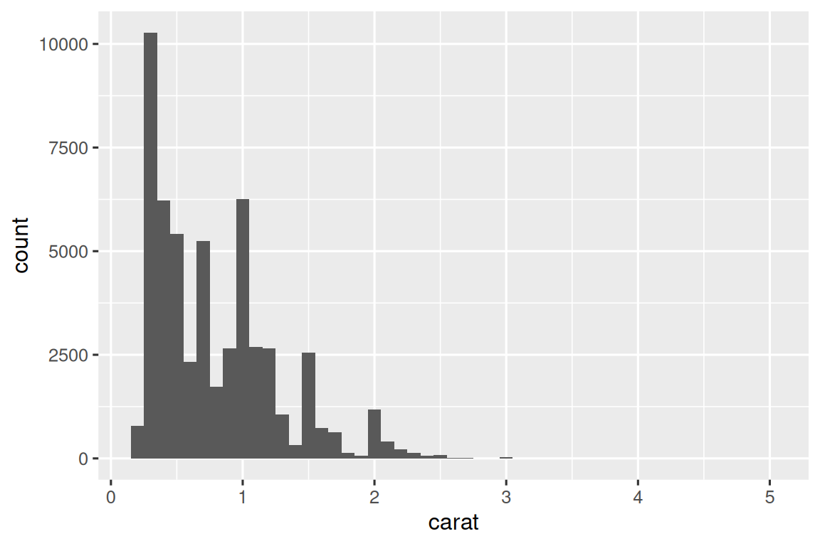
Note that histogram() returns a ggplot2 plot, meaning you can still add on additional components if you want. Just remember to switch from |> to +:
diamonds |>
  histogram(carat, 0.1) +
  labs(x = "Size (in carats)", y = "Number of diamonds")
25.4.1 More variables
It’s straightforward to add more variables to the mix. For example, maybe you want an easy way to eyeball whether or not a dataset is linear by overlaying a smooth line and a straight line:
# https://twitter.com/tyler_js_smith/status/1574377116988104704
linearity_check <- function(df, x, y) {
  df |>
    ggplot(aes(x = {{ x }}, y = {{ y }})) +
    geom_point() +
    geom_smooth(method = "loess", formula = y ~ x, color = "red", se = FALSE) +
    geom_smooth(method = "lm", formula = y ~ x, color = "blue", se = FALSE)
}

starwars |>
  filter(mass < 1000) |>
  linearity_check(mass, height)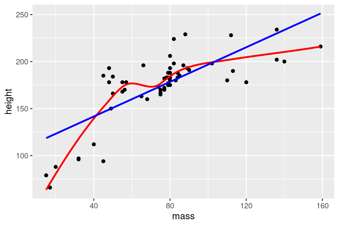
Or maybe you want an alternative to colored scatterplots for very large datasets where overplotting is a problem:
# https://twitter.com/ppaxisa/status/1574398423175921665
hex_plot <- function(df, x, y, z, bins = 20, fun = "mean") {
  df |>
    ggplot(aes(x = {{ x }}, y = {{ y }}, z = {{ z }})) +
    stat_summary_hex(
      aes(color = after_scale(fill)), # make border same color as fill
      bins = bins,
      fun = fun,
    )
}

diamonds |> hex_plot(carat, price, depth)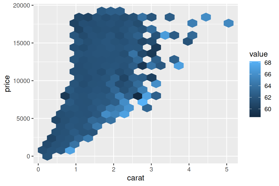
25.4.2 Combining with other tidyverse
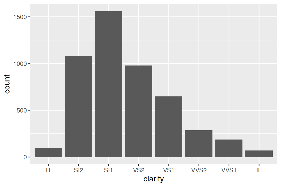
Some of the most useful helpers combine a dash of data manipulation with ggplot2. For example, if you might want to do a vertical bar chart where you automatically sort the bars in frequency order using fct_infreq(). Since the bar chart is vertical, we also need to reverse the usual order to get the highest values at the top:
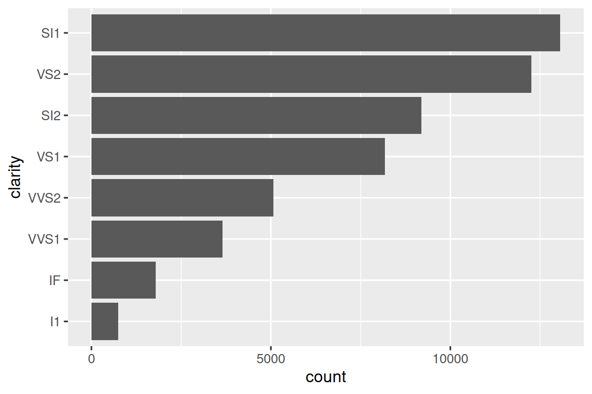
We have to use a new operator here, := (commonly referred to as the “walrus operator”), because we are generating the variable name based on user-supplied data. Variable names go on the left hand side of =, but R’s syntax doesn’t allow anything to the left of = except for a single literal name. To work around this problem, we use the special operator := which tidy evaluation treats in exactly the same way as =.
Or maybe you want to make it easy to draw a bar plot just for a subset of the data:
You can also get creative and display data summaries in other ways. You can find a cool application at https://gist.github.com/GShotwell/b19ef520b6d56f61a830fabb3454965b; it uses the axis labels to display the highest value. As you learn more about ggplot2, the power of your functions will continue to increase.
We’ll finish with a more complicated case: labelling the plots you create.
25.4.3 Labeling
Remember the histogram function we showed you earlier?
histogram <- function(df, var, binwidth = NULL) {
  df |>
    ggplot(aes(x = {{ var }})) +
    geom_histogram(binwidth = binwidth)
}
Wouldn’t it be nice if we could label the output with the variable and the bin width that was used? To do so, we’re going to have to go under the covers of tidy evaluation and use a function from the package we haven’t talked about yet: rlang. rlang is a low-level package that’s used by just about every other package in the tidyverse because it implements tidy evaluation (as well as many other useful tools).
To solve the labeling problem we can use rlang::englue(). This works similarly to str_glue(), so any value wrapped in { } will be inserted into the string. But it also understands {{ }}, which automatically inserts the appropriate variable name:
histogram <- function(df, var, binwidth) {
  label <- rlang::englue("A histogram of {{var}} with binwidth {binwidth}")

  df |>
    ggplot(aes(x = {{ var }})) +
    geom_histogram(binwidth = binwidth) +
    labs(title = label)
}

diamonds |> histogram(carat, 0.1)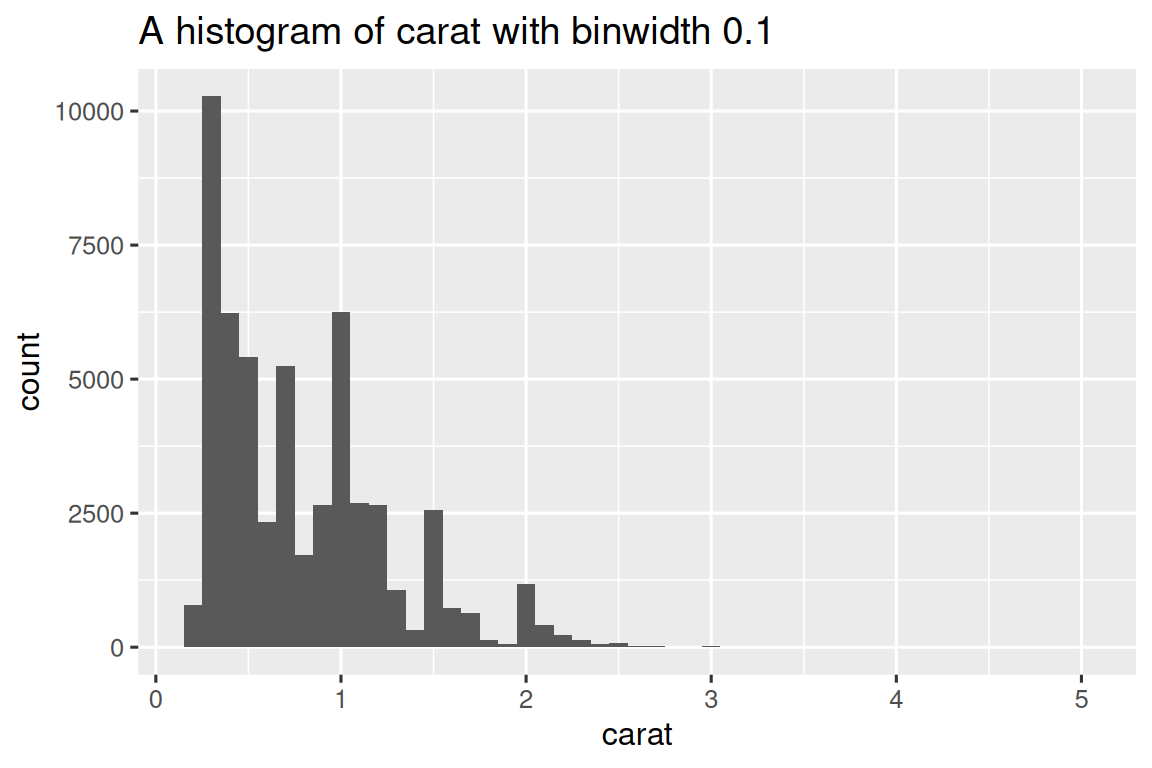
You can use the same approach in any other place where you want to supply a string in a ggplot2 plot.
25.4.4 Exercises
Build up a rich plotting function by incrementally implementing each of the steps below:
Draw a scatterplot given dataset and
xandyvariables.Add a line of best fit (i.e. a linear model with no standard errors).
Add a title.
25.5 Style
R doesn’t care what your function or arguments are called but the names make a big difference for humans. Ideally, the name of your function will be short, but clearly evoke what the function does. That’s hard! But it’s better to be clear than short, as RStudio’s autocomplete makes it easy to type long names.
Generally, function names should be verbs, and arguments should be nouns. There are some exceptions: nouns are ok if the function computes a very well known noun (i.e. mean() is better than compute_mean()), or accessing some property of an object (i.e. coef() is better than get_coefficients()). Use your best judgement and don’t be afraid to rename a function if you figure out a better name later.
# Too short
f()

# Not a verb, or descriptive
my_awesome_function()

# Long, but clear
impute_missing()
collapse_years()
R also doesn’t care about how you use white space in your functions but future readers will. Continue to follow the rules from Chapter 4. Additionally, function() should always be followed by squiggly brackets ({}), and the contents should be indented by an additional two spaces. This makes it easier to see the hierarchy in your code by skimming the left-hand margin.
# Missing extra two spaces
density <- function(color, facets, binwidth = 0.1) {
diamonds |>
  ggplot(aes(x = carat, y = after_stat(density), color = {{ color }})) +
  geom_freqpoly(binwidth = binwidth) +
  facet_wrap(vars({{ facets }}))
}

# Pipe indented incorrectly
density <- function(color, facets, binwidth = 0.1) {
  diamonds |>
  ggplot(aes(x = carat, y = after_stat(density), color = {{ color }})) +
  geom_freqpoly(binwidth = binwidth) +
  facet_wrap(vars({{ facets }}))
}
As you can see we recommend putting extra spaces inside of {{ }}. This makes it very obvious that something unusual is happening.
25.5.1 Exercises
-
Read the source code for each of the following two functions, puzzle out what they do, and then brainstorm better names.
f1 <- function(string, prefix) {
  str_sub(string, 1, str_length(prefix)) == prefix
}

f3 <- function(x, y) {
  rep(y, length.out = length(x))
}
Take a function that you’ve written recently and spend 5 minutes brainstorming a better name for it and its arguments.
Make a case for why
norm_r(),norm_d()etc. would be better thanrnorm(),dnorm(). Make a case for the opposite. How could you make the names even clearer?
25.6 Summary
In this chapter, you learned how to write functions for three useful scenarios: creating a vector, creating a data frame, or creating a plot. Along the way you saw many examples, which hopefully started to get your creative juices flowing, and gave you some ideas for where functions might help your analysis code.
We have only shown you the bare minimum to get started with functions and there’s much more to learn. A few places to learn more are:
- To learn more about programming with tidy evaluation, see useful recipes in programming with dplyr and programming with tidyr and learn more about the theory in What is data-masking and why do I need {{?.
- To learn more about reducing duplication in your ggplot2 code, read the Programming with ggplot2 chapter of the ggplot2 book.
- For more advice on function style, see the tidyverse style guide.
In the next chapter, we’ll dive into iteration which gives you further tools for reducing code duplication.