13 Numbers

13.1 Introduction

Numeric vectors are the backbone of data science, and you’ve already used them a bunch of times earlier in the book. Now it’s time to systematically survey what you can do with them in R, ensuring that you’re well situated to tackle any future problem involving numeric vectors.

We’ll start by giving you a couple of tools to make numbers if you have strings, and then going into a little more detail of count(). Then we’ll dive into various numeric transformations that pair well with mutate(), including more general transformations that can be applied to other types of vectors, but are often used with numeric vectors. We’ll finish off by covering the summary functions that pair well with summarize() and show you how they can also be used with mutate().

13.1.1 Prerequisites

This chapter mostly uses functions from base R, which are available without loading any packages. But we still need the tidyverse because we’ll use these base R functions inside of tidyverse functions like mutate() and filter(). Like in the last chapter, we’ll use real examples from nycflights13, as well as toy examples made with c() and tribble().

library(tidyverse)
library(nycflights13)

13.2 Making numbers

In most cases, you’ll get numbers already recorded in one of R’s numeric types: integer or double. In some cases, however, you’ll encounter them as strings, possibly because you’ve created them by pivoting from column headers or because something has gone wrong in your data import process.

readr provides two useful functions for parsing strings into numbers: parse_double() and parse_number(). Use parse_double() when you have numbers that have been written as strings:

x <- c("1.2", "5.6", "1e3")
parse_double(x)
#> [1]    1.2    5.6 1000.0

Use parse_number() when the string contains non-numeric text that you want to ignore. This is particularly useful for currency data and percentages:

x <- c("$1,234", "USD 3,513", "59%")
parse_number(x)
#> [1] 1234 3513   59

13.3 Counts

It’s surprising how much data science you can do with just counts and a little basic arithmetic, so dplyr strives to make counting as easy as possible with count(). This function is great for quick exploration and checks during analysis:

flights |> count(dest)
#> # A tibble: 105 × 2
#>   dest      n
#>   <chr> <int>
#> 1 ABQ     254
#> 2 ACK     265
#> 3 ALB     439
#> 4 ANC       8
#> 5 ATL   17215
#> 6 AUS    2439
#> # ℹ 99 more rows

(Despite the advice in Chapter 4, we usually put count() on a single line because it’s usually used at the console for a quick check that a calculation is working as expected.)

If you want to see the most common values, add sort = TRUE:

flights |> count(dest, sort = TRUE)
#> # A tibble: 105 × 2
#>   dest      n
#>   <chr> <int>
#> 1 ORD   17283
#> 2 ATL   17215
#> 3 LAX   16174
#> 4 BOS   15508
#> 5 MCO   14082
#> 6 CLT   14064
#> # ℹ 99 more rows

And remember that if you want to see all the values, you can use |> View() or |> print(n = Inf).

You can perform the same computation “by hand” with group_by(), summarize() and n(). This is useful because it allows you to compute other summaries at the same time:

flights |> 
  group_by(dest) |> 
  summarize(
    n = n(),
    delay = mean(arr_delay, na.rm = TRUE)
  )
#> # A tibble: 105 × 3
#>   dest      n delay
#>   <chr> <int> <dbl>
#> 1 ABQ     254  4.38
#> 2 ACK     265  4.85
#> 3 ALB     439 14.4 
#> 4 ANC       8 -2.5 
#> 5 ATL   17215 11.3 
#> 6 AUS    2439  6.02
#> # ℹ 99 more rows

n() is a special summary function that doesn’t take any arguments and instead accesses information about the “current” group. This means that it only works inside dplyr verbs:

n()
#> Error in `n()`:
#> ! Must only be used inside data-masking verbs like `mutate()`,
#>   `filter()`, and `group_by()`.

There are a couple of variants of n() and count() that you might find useful:

n_distinct(x) counts the number of distinct (unique) values of one or more variables. For example, we could figure out which destinations are served by the most carriers:

flights |> 
  group_by(dest) |> 
  summarize(carriers = n_distinct(carrier)) |> 
  arrange(desc(carriers))
#> # A tibble: 105 × 2
#>   dest  carriers
#>   <chr>    <int>
#> 1 ATL          7
#> 2 BOS          7
#> 3 CLT          7
#> 4 ORD          7
#> 5 TPA          7
#> 6 AUS          6
#> # ℹ 99 more rows

A weighted count is a sum. For example you could “count” the number of miles each plane flew:

flights |> 
  group_by(tailnum) |> 
  summarize(miles = sum(distance))
#> # A tibble: 4,044 × 2
#>   tailnum  miles
#>   <chr>    <dbl>
#> 1 D942DN    3418
#> 2 N0EGMQ  250866
#> 3 N10156  115966
#> 4 N102UW   25722
#> 5 N103US   24619
#> 6 N104UW   25157
#> # ℹ 4,038 more rows

Weighted counts are a common problem so count() has a wt argument that does the same thing:

flights |> count(tailnum, wt = distance)

You can count missing values by combining sum() and is.na(). In the flights dataset this represents flights that are cancelled:

flights |> 
  group_by(dest) |> 
  summarize(n_cancelled = sum(is.na(dep_time))) 
#> # A tibble: 105 × 2
#>   dest  n_cancelled
#>   <chr>       <int>
#> 1 ABQ             0
#> 2 ACK             0
#> 3 ALB            20
#> 4 ANC             0
#> 5 ATL           317
#> 6 AUS            21
#> # ℹ 99 more rows

13.3.1 Exercises

How can you use count() to count the number of rows with a missing value for a given variable?
Expand the following calls to count() to instead use group_by(), summarize(), and arrange():
1. flights |> count(dest, sort = TRUE)
2. flights |> count(tailnum, wt = distance)

13.4 Numeric transformations

Transformation functions work well with mutate() because their output is the same length as the input. The vast majority of transformation functions are already built into base R. It’s impractical to list them all so this section will show the most useful ones. As an example, while R provides all the trigonometric functions that you might dream of, we don’t list them here because they’re rarely needed for data science.

13.4.1 Arithmetic and recycling rules

We introduced the basics of arithmetic (+, -, *, /, ^) in Chapter 2 and have used them a bunch since. These functions don’t need a huge amount of explanation because they do what you learned in grade school. But we need to briefly talk about the recycling rules which determine what happens when the left and right hand sides have different lengths. This is important for operations like flights |> mutate(air_time = air_time / 60) because there are 336,776 numbers on the left of / but only one on the right.

R handles mismatched lengths by recycling, or repeating, the short vector. We can see this in operation more easily if we create some vectors outside of a data frame:

x <- c(1, 2, 10, 20)
x / 5
#> [1] 0.2 0.4 2.0 4.0
# is shorthand for
x / c(5, 5, 5, 5)
#> [1] 0.2 0.4 2.0 4.0

Generally, you only want to recycle single numbers (i.e. vectors of length 1), but R will recycle any shorter length vector. It usually (but not always) gives you a warning if the longer vector isn’t a multiple of the shorter:

x * c(1, 2)
#> [1]  1  4 10 40
x * c(1, 2, 3)
#> Warning in x * c(1, 2, 3): longer object length is not a multiple of shorter
#> object length
#> [1]  1  4 30 20

These recycling rules are also applied to logical comparisons (==, <, <=, >, >=, !=) and can lead to a surprising result if you accidentally use == instead of %in% and the data frame has an unfortunate number of rows. For example, take this code which attempts to find all flights in January and February:

flights |> 
  filter(month == c(1, 2))
#> # A tibble: 25,977 × 19
#>    year month   day dep_time sched_dep_time dep_delay arr_time sched_arr_time
#>   <int> <int> <int>    <int>          <int>     <dbl>    <int>          <int>
#> 1  2013     1     1      517            515         2      830            819
#> 2  2013     1     1      542            540         2      923            850
#> 3  2013     1     1      554            600        -6      812            837
#> 4  2013     1     1      555            600        -5      913            854
#> 5  2013     1     1      557            600        -3      838            846
#> 6  2013     1     1      558            600        -2      849            851
#> # ℹ 25,971 more rows
#> # ℹ 11 more variables: arr_delay <dbl>, carrier <chr>, flight <int>, …

The code runs without error, but it doesn’t return what you want. Because of the recycling rules it finds flights in odd numbered rows that departed in January and flights in even numbered rows that departed in February. And unfortunately there’s no warning because flights has an even number of rows.

To protect you from this type of silent failure, most tidyverse functions use a stricter form of recycling that only recycles single values. Unfortunately that doesn’t help here, or in many other cases, because the key computation is performed by the base R function ==, not filter().

13.4.2 Minimum and maximum

The arithmetic functions work with pairs of variables. Two closely related functions are pmin() and pmax(), which when given two or more variables will return the smallest or largest value in each row:

df <- tribble(
  ~x, ~y,
  1,  3,
  5,  2,
  7, NA,
)

df |> 
  mutate(
    min = pmin(x, y, na.rm = TRUE),
    max = pmax(x, y, na.rm = TRUE)
  )
#> # A tibble: 3 × 4
#>       x     y   min   max
#>   <dbl> <dbl> <dbl> <dbl>
#> 1     1     3     1     3
#> 2     5     2     2     5
#> 3     7    NA     7     7

Note that these are different to the summary functions min() and max() which take multiple observations and return a single value. You can tell that you’ve used the wrong form when all the minimums and all the maximums have the same value:

df |> 
  mutate(
    min = min(x, y, na.rm = TRUE),
    max = max(x, y, na.rm = TRUE)
  )
#> # A tibble: 3 × 4
#>       x     y   min   max
#>   <dbl> <dbl> <dbl> <dbl>
#> 1     1     3     1     7
#> 2     5     2     1     7
#> 3     7    NA     1     7

13.4.3 Modular arithmetic

Modular arithmetic is the technical name for the type of math you did before you learned about decimal places, i.e. division that yields a whole number and a remainder. In R, %/% does integer division and %% computes the remainder:

1:10 %/% 3
#>  [1] 0 0 1 1 1 2 2 2 3 3
1:10 %% 3
#>  [1] 1 2 0 1 2 0 1 2 0 1

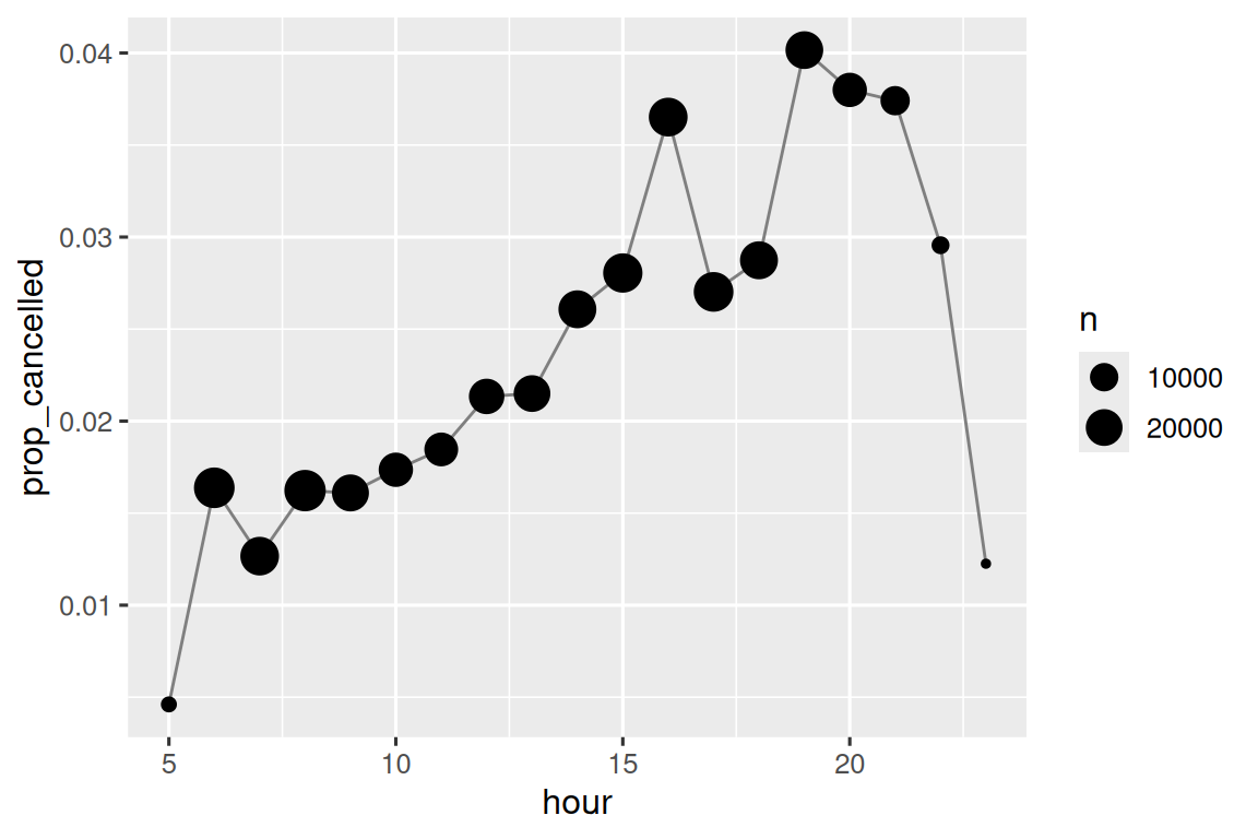
Modular arithmetic is handy for the flights dataset, because we can use it to unpack the sched_dep_time variable into hour and minute:

flights |> 
  mutate(
    hour = sched_dep_time %/% 100,
    minute = sched_dep_time %% 100,
    .keep = "used"
  )
#> # A tibble: 336,776 × 3
#>   sched_dep_time  hour minute
#>            <int> <dbl>  <dbl>
#> 1            515     5     15
#> 2            529     5     29
#> 3            540     5     40
#> 4            545     5     45
#> 5            600     6      0
#> 6            558     5     58
#> # ℹ 336,770 more rows

We can combine that with the mean(is.na(x)) trick from Section 12.4 to see how the proportion of cancelled flights varies over the course of the day. The results are shown in Figure 13.1.

flights |> 
  group_by(hour = sched_dep_time %/% 100) |> 
  summarize(prop_cancelled = mean(is.na(dep_time)), n = n()) |> 
  filter(hour > 1) |> 
  ggplot(aes(x = hour, y = prop_cancelled)) +
  geom_line(color = "grey50") + 
  geom_point(aes(size = n))

A line plot showing how proportion of cancelled flights changes over the course of the day. The proportion starts low at around 0.5% at 5am, then steadily increases over the course of the day until peaking at 4% at 7pm. The proportion of cancelled flights then drops rapidly getting down to around 1% by midnight. — Figure 13.1: A line plot with scheduled departure hour on the x-axis, and proportion of cancelled flights on the y-axis. Cancellations seem to accumulate over the course of the day until 8pm, very late flights are much less likely to be cancelled.

13.4.4 Logarithms

Logarithms are an incredibly useful transformation for dealing with data that ranges across multiple orders of magnitude and converting exponential growth to linear growth. In R, you have a choice of three logarithms: log() (the natural log, base e), log2() (base 2), and log10() (base 10). We recommend using log2() or log10(). log2() is easy to interpret because a difference of 1 on the log scale corresponds to doubling on the original scale and a difference of -1 corresponds to halving; whereas log10() is easy to back-transform because (e.g.) 3 is 10^3 = 1000. The inverse of log() is exp(); to compute the inverse of log2() or log10() you’ll need to use 2^ or 10^.

13.4.5 Rounding

Use round(x) to round a number to the nearest integer:

round(123.456)
#> [1] 123

You can control the precision of the rounding with the second argument, digits. round(x, digits) rounds to the nearest 10^-n so digits = 2 will round to the nearest 0.01. This definition is useful because it implies round(x, -3) will round to the nearest thousand, which indeed it does:

round(123.456, 2)  # two digits
#> [1] 123.46
round(123.456, 1)  # one digit
#> [1] 123.5
round(123.456, -1) # round to nearest ten
#> [1] 120
round(123.456, -2) # round to nearest hundred
#> [1] 100

There’s one weirdness with round() that seems surprising at first glance:

round(c(1.5, 2.5))
#> [1] 2 2

round() uses what’s known as “round half to even” or Banker’s rounding: if a number is half way between two integers, it will be rounded to the even integer. This is a good strategy because it keeps the rounding unbiased: half of all 0.5s are rounded up, and half are rounded down.

round() is paired with floor() which always rounds down and ceiling() which always rounds up:

x <- 123.456

floor(x)
#> [1] 123
ceiling(x)
#> [1] 124

These functions don’t have a digits argument, so you can instead scale down, round, and then scale back up:

# Round down to nearest two digits
floor(x / 0.01) * 0.01
#> [1] 123.45
# Round up to nearest two digits
ceiling(x / 0.01) * 0.01
#> [1] 123.46

You can use the same technique if you want to round() to a multiple of some other number:

# Round to nearest multiple of 4
round(x / 4) * 4
#> [1] 124

# Round to nearest 0.25
round(x / 0.25) * 0.25
#> [1] 123.5

13.4.6 Cutting numbers into ranges

Use cut()¹ to break up (aka bin) a numeric vector into discrete buckets:

x <- c(1, 2, 5, 10, 15, 20)
cut(x, breaks = c(0, 5, 10, 15, 20))
#> [1] (0,5]   (0,5]   (0,5]   (5,10]  (10,15] (15,20]
#> Levels: (0,5] (5,10] (10,15] (15,20]

The breaks don’t need to be evenly spaced:

cut(x, breaks = c(0, 5, 10, 100))
#> [1] (0,5]    (0,5]    (0,5]    (5,10]   (10,100] (10,100]
#> Levels: (0,5] (5,10] (10,100]

You can optionally supply your own labels. Note that there should be one less labels than breaks.

cut(x, 
  breaks = c(0, 5, 10, 15, 20), 
  labels = c("sm", "md", "lg", "xl")
)
#> [1] sm sm sm md lg xl
#> Levels: sm md lg xl

Any values outside of the range of the breaks will become NA:

y <- c(NA, -10, 5, 10, 30)
cut(y, breaks = c(0, 5, 10, 15, 20))
#> [1] <NA>   <NA>   (0,5]  (5,10] <NA>  
#> Levels: (0,5] (5,10] (10,15] (15,20]

See the documentation for other useful arguments like right and include.lowest, which control if the intervals are [a, b) or (a, b] and if the lowest interval should be [a, b].

13.4.7 Cumulative and rolling aggregates

Base R provides cumsum(), cumprod(), cummin(), cummax() for running, or cumulative, sums, products, mins and maxes. dplyr provides cummean() for cumulative means. Cumulative sums tend to come up the most in practice:

x <- 1:10
cumsum(x)
#>  [1]  1  3  6 10 15 21 28 36 45 55

If you need more complex rolling or sliding aggregates, try the slider package.

13.4.8 Exercises

Explain in words what each line of the code used to generate Figure 13.1 does.
What trigonometric functions does R provide? Guess some names and look up the documentation. Do they use degrees or radians?
Currently dep_time and sched_dep_time are convenient to look at, but hard to compute with because they’re not really continuous numbers. You can see the basic problem by running the code below: there’s a gap between each hour.
```
flights |> 
  filter(month == 1, day == 1) |> 
  ggplot(aes(x = sched_dep_time, y = dep_delay)) +
  geom_point()
```
Convert them to a more truthful representation of time (either fractional hours or minutes since midnight).
Round dep_time and arr_time to the nearest five minutes.

13.5 General transformations

The following sections describe some general transformations which are often used with numeric vectors, but can be applied to all other column types.

13.5.1 Ranks

dplyr provides a number of ranking functions inspired by SQL, but you should always start with dplyr::min_rank(). It uses the typical method for dealing with ties, e.g., 1st, 2nd, 2nd, 4th.

x <- c(1, 2, 2, 3, 4, NA)
min_rank(x)
#> [1]  1  2  2  4  5 NA

Note that the smallest values get the lowest ranks; use desc(x) to give the largest values the smallest ranks:

min_rank(desc(x))
#> [1]  5  3  3  2  1 NA

If min_rank() doesn’t do what you need, look at the variants dplyr::row_number(), dplyr::dense_rank(), dplyr::percent_rank(), and dplyr::cume_dist(). See the documentation for details.

df <- tibble(x = x)
df |> 
  mutate(
    row_number = row_number(x),
    dense_rank = dense_rank(x),
    percent_rank = percent_rank(x),
    cume_dist = cume_dist(x)
  )
#> # A tibble: 6 × 5
#>       x row_number dense_rank percent_rank cume_dist
#>   <dbl>      <int>      <int>        <dbl>     <dbl>
#> 1     1          1          1         0          0.2
#> 2     2          2          2         0.25       0.6
#> 3     2          3          2         0.25       0.6
#> 4     3          4          3         0.75       0.8
#> 5     4          5          4         1          1  
#> 6    NA         NA         NA        NA         NA

You can achieve many of the same results by picking the appropriate ties.method argument to base R’s rank(); you’ll probably also want to set na.last = "keep" to keep NAs as NA.

row_number() can also be used without any arguments when inside a dplyr verb. In this case, it’ll give the number of the “current” row. When combined with %% or %/% this can be a useful tool for dividing data into similarly sized groups:

df <- tibble(id = 1:10)

df |> 
  mutate(
    row0 = row_number() - 1,
    three_groups = row0 %% 3,
    three_in_each_group = row0 %/% 3
  )
#> # A tibble: 10 × 4
#>      id  row0 three_groups three_in_each_group
#>   <int> <dbl>        <dbl>               <dbl>
#> 1     1     0            0                   0
#> 2     2     1            1                   0
#> 3     3     2            2                   0
#> 4     4     3            0                   1
#> 5     5     4            1                   1
#> 6     6     5            2                   1
#> # ℹ 4 more rows

13.5.2 Offsets

dplyr::lead() and dplyr::lag() allow you to refer the values just before or just after the “current” value. They return a vector of the same length as the input, padded with NAs at the start or end:

x <- c(2, 5, 11, 11, 19, 35)
lag(x)
#> [1] NA  2  5 11 11 19
lead(x)
#> [1]  5 11 11 19 35 NA

x - lag(x) gives you the difference between the current and previous value.
```
x - lag(x)
#> [1] NA  3  6  0  8 16
```

x == lag(x) tells you when the current value changes.

x == lag(x)
#> [1]    NA FALSE FALSE  TRUE FALSE FALSE

You can lead or lag by more than one position by using the second argument, n.

13.5.3 Consecutive identifiers

Sometimes you want to start a new group every time some event occurs. For example, when you’re looking at website data, it’s common to want to break up events into sessions, where you begin a new session after gap of more than x minutes since the last activity. For example, imagine you have the times when someone visited a website:

events <- tibble(
  time = c(0, 1, 2, 3, 5, 10, 12, 15, 17, 19, 20, 27, 28, 30)
)

And you’ve computed the time between each event, and figured out if there’s a gap that’s big enough to qualify:

events <- events |> 
  mutate(
    diff = time - lag(time, default = first(time)),
    has_gap = diff >= 5
  )
events
#> # A tibble: 14 × 3
#>    time  diff has_gap
#>   <dbl> <dbl> <lgl>  
#> 1     0     0 FALSE  
#> 2     1     1 FALSE  
#> 3     2     1 FALSE  
#> 4     3     1 FALSE  
#> 5     5     2 FALSE  
#> 6    10     5 TRUE   
#> # ℹ 8 more rows

But how do we go from that logical vector to something that we can group_by()? cumsum(), from Section 13.4.7, comes to the rescue as gap, i.e. has_gap is TRUE, will increment group by one (Section 12.4.2):

events |> mutate(
  group = cumsum(has_gap)
)
#> # A tibble: 14 × 4
#>    time  diff has_gap group
#>   <dbl> <dbl> <lgl>   <int>
#> 1     0     0 FALSE       0
#> 2     1     1 FALSE       0
#> 3     2     1 FALSE       0
#> 4     3     1 FALSE       0
#> 5     5     2 FALSE       0
#> 6    10     5 TRUE        1
#> # ℹ 8 more rows

Another approach for creating grouping variables is consecutive_id(), which starts a new group every time one of its arguments changes. For example, inspired by this stackoverflow question, imagine you have a data frame with a bunch of repeated values:

df <- tibble(
  x = c("a", "a", "a", "b", "c", "c", "d", "e", "a", "a", "b", "b"),
  y = c(1, 2, 3, 2, 4, 1, 3, 9, 4, 8, 10, 199)
)

If you want to keep the first row from each repeated x, you could use group_by(), consecutive_id(), and slice_head():

df |> 
  group_by(id = consecutive_id(x)) |> 
  slice_head(n = 1)
#> # A tibble: 7 × 3
#> # Groups:   id [7]
#>   x         y    id
#>   <chr> <dbl> <int>
#> 1 a         1     1
#> 2 b         2     2
#> 3 c         4     3
#> 4 d         3     4
#> 5 e         9     5
#> 6 a         4     6
#> # ℹ 1 more row

13.5.4 Exercises

Find the 10 most delayed flights using a ranking function. How do you want to handle ties? Carefully read the documentation for min_rank().
Which plane (tailnum) has the worst on-time record?
What time of day should you fly if you want to avoid delays as much as possible?
What does flights |> group_by(dest) |> filter(row_number() < 4) do? What does flights |> group_by(dest) |> filter(row_number(dep_delay) < 4) do?
For each destination, compute the total minutes of delay. For each flight, compute the proportion of the total delay for its destination.
Delays are typically temporally correlated: even once the problem that caused the initial delay has been resolved, later flights are delayed to allow earlier flights to leave. Using lag(), explore how the average flight delay for an hour is related to the average delay for the previous hour.
```
flights |> 
  mutate(hour = dep_time %/% 100) |> 
  group_by(year, month, day, hour) |> 
  summarize(
    dep_delay = mean(dep_delay, na.rm = TRUE),
    n = n(),
    .groups = "drop"
  ) |> 
  filter(n > 5)
```
Look at each destination. Can you find flights that are suspiciously fast (i.e. flights that represent a potential data entry error)? Compute the air time of a flight relative to the shortest flight to that destination. Which flights were most delayed in the air?
Find all destinations that are flown by at least two carriers. Use those destinations to come up with a relative ranking of the carriers based on their performance for the same destination.

13.6 Numeric summaries

Just using the counts, means, and sums that we’ve introduced already can get you a long way, but R provides many other useful summary functions. Here is a selection that you might find useful.

13.6.1 Center

So far, we’ve mostly used mean() to summarize the center of a vector of values. As we’ve seen in Section 3.6, because the mean is the sum divided by the count, it is sensitive to even just a few unusually high or low values. An alternative is to use the median(), which finds a value that lies in the “middle” of the vector, i.e. 50% of the values is above it and 50% are below it. Depending on the shape of the distribution of the variable you’re interested in, mean or median might be a better measure of center. For example, for symmetric distributions we generally report the mean while for skewed distributions we usually report the median.

Figure 13.2 compares the mean vs. the median departure delay (in minutes) for each destination. The median delay is always smaller than the mean delay because flights sometimes leave multiple hours late, but never leave multiple hours early.

flights |>
  group_by(year, month, day) |>
  summarize(
    mean = mean(dep_delay, na.rm = TRUE),
    median = median(dep_delay, na.rm = TRUE),
    n = n(),
    .groups = "drop"
  ) |> 
  ggplot(aes(x = mean, y = median)) + 
  geom_abline(slope = 1, intercept = 0, color = "white", linewidth = 2) +
  geom_point()

All points fall below a 45° line, meaning that the median delay is always less than the mean delay. Most points are clustered in a dense region of mean [0, 20] and median [-5, 5]. As the mean delay increases, the spread of the median also increases. There are two outlying points with mean ~60, median ~30, and mean ~85, median ~55. — Figure 13.2: A scatterplot showing the differences of summarizing daily departure delay with median instead of mean.

You might also wonder about the mode, or the most common value. This is a summary that only works well for very simple cases (which is why you might have learned about it in high school), but it doesn’t work well for many real datasets. If the data is discrete, there may be multiple most common values, and if the data is continuous, there might be no most common value because every value is ever so slightly different. For these reasons, the mode tends not to be used by statisticians and there’s no mode function included in base R².

13.6.2 Minimum, maximum, and quantiles

What if you’re interested in locations other than the center? min() and max() will give you the largest and smallest values. Another powerful tool is quantile() which is a generalization of the median: quantile(x, 0.25) will find the value of x that is greater than 25% of the values, quantile(x, 0.5) is equivalent to the median, and quantile(x, 0.95) will find the value that’s greater than 95% of the values.

For the flights data, you might want to look at the 95% quantile of delays rather than the maximum, because it will ignore the 5% of most delayed flights which can be quite extreme.

flights |>
  group_by(year, month, day) |>
  summarize(
    max = max(dep_delay, na.rm = TRUE),
    q95 = quantile(dep_delay, 0.95, na.rm = TRUE),
    .groups = "drop"
  )
#> # A tibble: 365 × 5
#>    year month   day   max   q95
#>   <int> <int> <int> <dbl> <dbl>
#> 1  2013     1     1   853  70.1
#> 2  2013     1     2   379  85  
#> 3  2013     1     3   291  68  
#> 4  2013     1     4   288  60  
#> 5  2013     1     5   327  41  
#> 6  2013     1     6   202  51  
#> # ℹ 359 more rows

13.6.3 Spread

Sometimes you’re not so interested in where the bulk of the data lies, but in how it is spread out. Two commonly used summaries are the standard deviation, sd(x), and the inter-quartile range, IQR(). We won’t explain sd() here since you’re probably already familiar with it, but IQR() might be new — it’s quantile(x, 0.75) - quantile(x, 0.25) and gives you the range that contains the middle 50% of the data.

We can use this to reveal a small oddity in the flights data. You might expect the spread of the distance between origin and destination to be zero, since airports are always in the same place. But the code below reveals a data oddity for airport EGE:

flights |> 
  group_by(origin, dest) |> 
  summarize(
    distance_iqr = IQR(distance), 
    n = n(),
    .groups = "drop"
  ) |> 
  filter(distance_iqr > 0)
#> # A tibble: 2 × 4
#>   origin dest  distance_iqr     n
#>   <chr>  <chr>        <dbl> <int>
#> 1 EWR    EGE              1   110
#> 2 JFK    EGE              1   103

13.6.4 Distributions

It’s worth remembering that all of the summary statistics described above are a way of reducing the distribution down to a single number. This means that they’re fundamentally reductive, and if you pick the wrong summary, you can easily miss important differences between groups. That’s why it’s always a good idea to visualize the distribution before committing to your summary statistics.

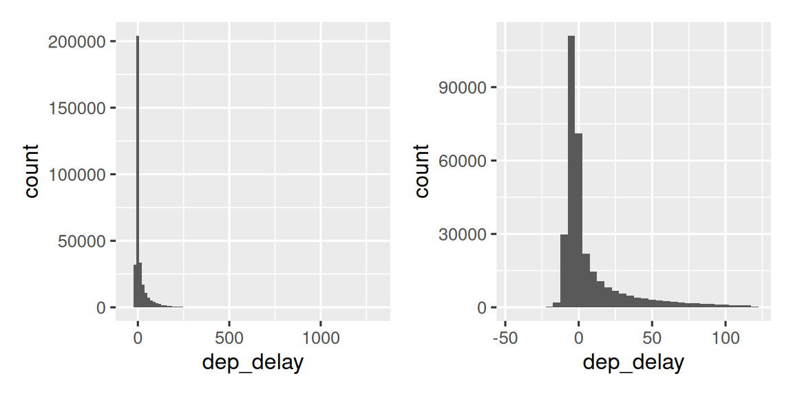
Figure 13.3 shows the overall distribution of departure delays. The distribution is so skewed that we have to zoom in to see the bulk of the data. This suggests that the mean is unlikely to be a good summary and we might prefer the median instead.

Two histograms of `dep_delay`. On the left, it's very hard to see any pattern except that there's a very large spike around zero, the bars rapidly decay in height, and for most of the plot, you can't see any bars because they are too short to see. On the right, where we've discarded delays of greater than two hours, we can see that the spike occurs slightly below zero (i.e. most flights leave a couple of minutes early), but there's still a very steep decay after that. — Figure 13.3: (Left) The histogram of the full data is extremely skewed making it hard to get any details. (Right) Zooming into delays of less than two hours makes it possible to see what’s happening with the bulk of the observations.

It’s also a good idea to check that distributions for subgroups resemble the whole. In the following plot 365 frequency polygons of dep_delay, one for each day, are overlaid. The distributions seem to follow a common pattern, suggesting it’s fine to use the same summary for each day.

flights |>
  filter(dep_delay < 120) |> 
  ggplot(aes(x = dep_delay, group = interaction(day, month))) + 
  geom_freqpoly(binwidth = 5, alpha = 1/5)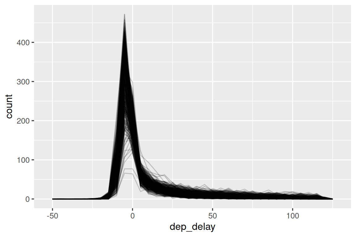

The distribution of `dep_delay` is highly right skewed with a strong peak slightly less than 0. The 365 frequency polygons are mostly overlapping forming a thick black band.

Don’t be afraid to explore your own custom summaries specifically tailored for the data that you’re working with. In this case, that might mean separately summarizing the flights that left early vs. the flights that left late, or given that the values are so heavily skewed, you might try a log-transformation. Finally, don’t forget what you learned in Section 3.6: whenever creating numerical summaries, it’s a good idea to include the number of observations in each group.

13.6.5 Positions

There’s one final type of summary that’s useful for numeric vectors, but also works with every other type of value: extracting a value at a specific position: first(x), last(x), and nth(x, n).

For example, we can find the first, fifth and last departure for each day:

flights |> 
  group_by(year, month, day) |> 
  summarize(
    first_dep = first(dep_time, na_rm = TRUE), 
    fifth_dep = nth(dep_time, 5, na_rm = TRUE),
    last_dep = last(dep_time, na_rm = TRUE)
  )
#> `summarise()` has grouped output by 'year', 'month'. You can override using
#> the `.groups` argument.
#> # A tibble: 365 × 6
#> # Groups:   year, month [12]
#>    year month   day first_dep fifth_dep last_dep
#>   <int> <int> <int>     <int>     <int>    <int>
#> 1  2013     1     1       517       554     2356
#> 2  2013     1     2        42       535     2354
#> 3  2013     1     3        32       520     2349
#> 4  2013     1     4        25       531     2358
#> 5  2013     1     5        14       534     2357
#> 6  2013     1     6        16       555     2355
#> # ℹ 359 more rows

(NB: Because dplyr functions use _ to separate components of function and arguments names, these functions use na_rm instead of na.rm.)

If you’re familiar with [, which we’ll come back to in Section 27.2, you might wonder if you ever need these functions. There are three reasons: the default argument allows you to provide a default if the specified position doesn’t exist, the order_by argument allows you to locally override the order of the rows, and the na_rm argument allows you to drop missing values.

Extracting values at positions is complementary to filtering on ranks. Filtering gives you all variables, with each observation in a separate row:

flights |> 
  group_by(year, month, day) |> 
  mutate(r = min_rank(sched_dep_time)) |> 
  filter(r %in% c(1, max(r)))
#> # A tibble: 1,195 × 20
#> # Groups:   year, month, day [365]
#>    year month   day dep_time sched_dep_time dep_delay arr_time sched_arr_time
#>   <int> <int> <int>    <int>          <int>     <dbl>    <int>          <int>
#> 1  2013     1     1      517            515         2      830            819
#> 2  2013     1     1     2353           2359        -6      425            445
#> 3  2013     1     1     2353           2359        -6      418            442
#> 4  2013     1     1     2356           2359        -3      425            437
#> 5  2013     1     2       42           2359        43      518            442
#> 6  2013     1     2      458            500        -2      703            650
#> # ℹ 1,189 more rows
#> # ℹ 12 more variables: arr_delay <dbl>, carrier <chr>, flight <int>, …

13.6.6 With `mutate()`

As the names suggest, the summary functions are typically paired with summarize(). However, because of the recycling rules we discussed in Section 13.4.1 they can also be usefully paired with mutate(), particularly when you want do some sort of group standardization. For example:

x / sum(x) calculates the proportion of a total.
(x - mean(x)) / sd(x) computes a Z-score (standardized to mean 0 and sd 1).
(x - min(x)) / (max(x) - min(x)) standardizes to range [0, 1].
x / first(x) computes an index based on the first observation.

13.6.7 Exercises

Brainstorm at least 5 different ways to assess the typical delay characteristics of a group of flights. When is mean() useful? When is median() useful? When might you want to use something else? Should you use arrival delay or departure delay? Why might you want to use data from planes?
Which destinations show the greatest variation in air speed?
Create a plot to further explore the adventures of EGE. Can you find any evidence that the airport moved locations? Can you find another variable that might explain the difference?

13.7 Summary

You’re already familiar with many tools for working with numbers, and after reading this chapter you now know how to use them in R. You’ve also learned a handful of useful general transformations that are commonly, but not exclusively, applied to numeric vectors like ranks and offsets. Finally, you worked through a number of numeric summaries, and discussed a few of the statistical challenges that you should consider.

Over the next two chapters, we’ll dive into working with strings with the stringr package. Strings are a big topic so they get two chapters, one on the fundamentals of strings and one on regular expressions.

ggplot2 provides some helpers for common cases in cut_interval(), cut_number(), and cut_width(). ggplot2 is an admittedly weird place for these functions to live, but they are useful as part of histogram computation and were written before any other parts of the tidyverse existed.↩︎
The mode() function does something quite different!↩︎