12 Logical vectors

12.1 Introduction

In this chapter, you’ll learn tools for working with logical vectors. Logical vectors are the simplest type of vector because each element can only be one of three possible values: TRUE, FALSE, and NA. It’s relatively rare to find logical vectors in your raw data, but you’ll create and manipulate them in the course of almost every analysis.

We’ll begin by discussing the most common way of creating logical vectors: with numeric comparisons. Then you’ll learn about how you can use Boolean algebra to combine different logical vectors, as well as some useful summaries. We’ll finish off with if_else() and case_when(), two useful functions for making conditional changes powered by logical vectors.

12.1.1 Prerequisites

Most of the functions you’ll learn about in this chapter are provided by base R, so we don’t need the tidyverse, but we’ll still load it so we can use mutate(), filter(), and friends to work with data frames. We’ll also continue to draw examples from the nycflights13::flights dataset.

library(tidyverse)
library(nycflights13)

However, as we start to cover more tools, there won’t always be a perfect real example. So we’ll start making up some dummy data with c():

x <- c(1, 2, 3, 5, 7, 11, 13)
x * 2
#> [1]  2  4  6 10 14 22 26

This makes it easier to explain individual functions at the cost of making it harder to see how it might apply to your data problems. Just remember that any manipulation we do to a free-floating vector, you can do to a variable inside a data frame with mutate() and friends.

df <- tibble(x)
df |> 
  mutate(y = x * 2)
#> # A tibble: 7 × 2
#>       x     y
#>   <dbl> <dbl>
#> 1     1     2
#> 2     2     4
#> 3     3     6
#> 4     5    10
#> 5     7    14
#> 6    11    22
#> # ℹ 1 more row

12.2 Comparisons

A very common way to create a logical vector is via a numeric comparison with <, <=, >, >=, !=, and ==. So far, we’ve mostly created logical variables transiently within filter() — they are computed, used, and then thrown away. For example, the following filter finds all daytime departures that arrive roughly on time:

flights |> 
  filter(dep_time > 600 & dep_time < 2000 & abs(arr_delay) < 20)
#> # A tibble: 172,286 × 19
#>    year month   day dep_time sched_dep_time dep_delay arr_time sched_arr_time
#>   <int> <int> <int>    <int>          <int>     <dbl>    <int>          <int>
#> 1  2013     1     1      601            600         1      844            850
#> 2  2013     1     1      602            610        -8      812            820
#> 3  2013     1     1      602            605        -3      821            805
#> 4  2013     1     1      606            610        -4      858            910
#> 5  2013     1     1      606            610        -4      837            845
#> 6  2013     1     1      607            607         0      858            915
#> # ℹ 172,280 more rows
#> # ℹ 11 more variables: arr_delay <dbl>, carrier <chr>, flight <int>, …

It’s useful to know that this is a shortcut and you can explicitly create the underlying logical variables with mutate():

flights |> 
  mutate(
    daytime = dep_time > 600 & dep_time < 2000,
    approx_ontime = abs(arr_delay) < 20,
    .keep = "used"
  )
#> # A tibble: 336,776 × 4
#>   dep_time arr_delay daytime approx_ontime
#>      <int>     <dbl> <lgl>   <lgl>        
#> 1      517        11 FALSE   TRUE         
#> 2      533        20 FALSE   FALSE        
#> 3      542        33 FALSE   FALSE        
#> 4      544       -18 FALSE   TRUE         
#> 5      554       -25 FALSE   FALSE        
#> 6      554        12 FALSE   TRUE         
#> # ℹ 336,770 more rows

This is particularly useful for more complicated logic because naming the intermediate steps makes it easier to both read your code and check that each step has been computed correctly.

All up, the initial filter is equivalent to:

flights |> 
  mutate(
    daytime = dep_time > 600 & dep_time < 2000,
    approx_ontime = abs(arr_delay) < 20,
  ) |> 
  filter(daytime & approx_ontime)

12.2.1 Floating point comparison

Beware of using == with numbers. For example, it looks like this vector contains the numbers 1 and 2:

x <- c(1 / 49 * 49, sqrt(2) ^ 2)
x
#> [1] 1 2

But if you test them for equality, you get FALSE:

x == c(1, 2)
#> [1] FALSE FALSE

What’s going on? Computers store numbers with a fixed number of decimal places so there’s no way to exactly represent 1/49 or sqrt(2) and subsequent computations will be very slightly off. We can see the exact values by calling print() with the digits¹ argument:

print(x, digits = 16)
#> [1] 0.9999999999999999 2.0000000000000004

You can see why R defaults to rounding these numbers; they really are very close to what you expect.

Now that you’ve seen why == is failing, what can you do about it? One option is to use dplyr::near() which ignores small differences:

near(x, c(1, 2))
#> [1] TRUE TRUE

12.2.2 Missing values

Missing values represent the unknown so they are “contagious”: almost any operation involving an unknown value will also be unknown:

NA > 5
#> [1] NA
10 == NA
#> [1] NA

The most confusing result is this one:

NA == NA
#> [1] NA

It’s easiest to understand why this is true if we artificially supply a little more context:

# We don't know how old Mary is
age_mary <- NA

# We don't know how old John is
age_john <- NA

# Are Mary and John the same age?
age_mary == age_john
#> [1] NA
# We don't know!

So if you want to find all flights where dep_time is missing, the following code doesn’t work because dep_time == NA will yield NA for every single row, and filter() automatically drops missing values:

flights |> 
  filter(dep_time == NA)
#> # A tibble: 0 × 19
#> # ℹ 19 variables: year <int>, month <int>, day <int>, dep_time <int>,
#> #   sched_dep_time <int>, dep_delay <dbl>, arr_time <int>, …

Instead we’ll need a new tool: is.na().

12.2.3 `is.na()`

is.na(x) works with any type of vector and returns TRUE for missing values and FALSE for everything else:

is.na(c(TRUE, NA, FALSE))
#> [1] FALSE  TRUE FALSE
is.na(c(1, NA, 3))
#> [1] FALSE  TRUE FALSE
is.na(c("a", NA, "b"))
#> [1] FALSE  TRUE FALSE

We can use is.na() to find all the rows with a missing dep_time:

flights |> 
  filter(is.na(dep_time))
#> # A tibble: 8,255 × 19
#>    year month   day dep_time sched_dep_time dep_delay arr_time sched_arr_time
#>   <int> <int> <int>    <int>          <int>     <dbl>    <int>          <int>
#> 1  2013     1     1       NA           1630        NA       NA           1815
#> 2  2013     1     1       NA           1935        NA       NA           2240
#> 3  2013     1     1       NA           1500        NA       NA           1825
#> 4  2013     1     1       NA            600        NA       NA            901
#> 5  2013     1     2       NA           1540        NA       NA           1747
#> 6  2013     1     2       NA           1620        NA       NA           1746
#> # ℹ 8,249 more rows
#> # ℹ 11 more variables: arr_delay <dbl>, carrier <chr>, flight <int>, …

is.na() can also be useful in arrange(). arrange() usually puts all the missing values at the end but you can override this default by first sorting by is.na():

flights |> 
  filter(month == 1, day == 1) |> 
  arrange(dep_time)
#> # A tibble: 842 × 19
#>    year month   day dep_time sched_dep_time dep_delay arr_time sched_arr_time
#>   <int> <int> <int>    <int>          <int>     <dbl>    <int>          <int>
#> 1  2013     1     1      517            515         2      830            819
#> 2  2013     1     1      533            529         4      850            830
#> 3  2013     1     1      542            540         2      923            850
#> 4  2013     1     1      544            545        -1     1004           1022
#> 5  2013     1     1      554            600        -6      812            837
#> 6  2013     1     1      554            558        -4      740            728
#> # ℹ 836 more rows
#> # ℹ 11 more variables: arr_delay <dbl>, carrier <chr>, flight <int>, …

flights |> 
  filter(month == 1, day == 1) |> 
  arrange(desc(is.na(dep_time)), dep_time)
#> # A tibble: 842 × 19
#>    year month   day dep_time sched_dep_time dep_delay arr_time sched_arr_time
#>   <int> <int> <int>    <int>          <int>     <dbl>    <int>          <int>
#> 1  2013     1     1       NA           1630        NA       NA           1815
#> 2  2013     1     1       NA           1935        NA       NA           2240
#> 3  2013     1     1       NA           1500        NA       NA           1825
#> 4  2013     1     1       NA            600        NA       NA            901
#> 5  2013     1     1      517            515         2      830            819
#> 6  2013     1     1      533            529         4      850            830
#> # ℹ 836 more rows
#> # ℹ 11 more variables: arr_delay <dbl>, carrier <chr>, flight <int>, …

We’ll come back to cover missing values in more depth in Chapter 18.

12.2.4 Exercises

How does dplyr::near() work? Type near to see the source code. Is sqrt(2)^2 near 2?
Use mutate(), is.na(), and count() together to describe how the missing values in dep_time, sched_dep_time and dep_delay are connected.

12.3 Boolean algebra

Once you have multiple logical vectors, you can combine them together using Boolean algebra. In R, & is “and”, | is “or”, ! is “not”, and xor() is exclusive or². For example, df |> filter(!is.na(x)) finds all rows where x is not missing and df |> filter(x < -10 | x > 0) finds all rows where x is smaller than -10 or bigger than 0. Figure 12.1 shows the complete set of Boolean operations and how they work.

Six Venn diagrams, each explaining a given logical operator. The circles (sets) in each of the Venn diagrams represent x and y. 1. y & !x is y but none of x; x & y is the intersection of x and y; x & !y is x but none of y; x is all of x none of y; xor(x, y) is everything except the intersection of x and y; y is all of y and none of x; and x | y is everything. — Figure 12.1: The complete set of Boolean operations. 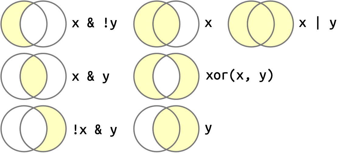`x` is the left-hand circle, `y` is the right-hand circle, and the shaded region show which parts each operator selects.

As well as & and |, R also has && and ||. Don’t use them in dplyr functions! These are called short-circuiting operators and only ever return a single TRUE or FALSE. They’re important for programming, not data science.

12.3.1 Missing values

The rules for missing values in Boolean algebra are a little tricky to explain because they seem inconsistent at first glance:

df <- tibble(x = c(TRUE, FALSE, NA))

df |> 
  mutate(
    and = x & NA,
    or = x | NA
  )
#> # A tibble: 3 × 3
#>   x     and   or   
#>   <lgl> <lgl> <lgl>
#> 1 TRUE  NA    TRUE 
#> 2 FALSE FALSE NA   
#> 3 NA    NA    NA

To understand what’s going on, think about NA | TRUE (NA or TRUE). A missing value in a logical vector means that the value could either be TRUE or FALSE. TRUE | TRUE and FALSE | TRUE are both TRUE because at least one of them is TRUE. NA | TRUE must also be TRUE because NA can either be TRUE or FALSE. However, NA | FALSE is NA because we don’t know if NA is TRUE or FALSE. Similar reasoning applies with NA & FALSE.

12.3.2 Order of operations

Note that the order of operations doesn’t work like English. Take the following code that finds all flights that departed in November or December:

flights |> 
   filter(month == 11 | month == 12)

You might be tempted to write it like you’d say in English: “Find all flights that departed in November or December.”:

flights |> 
   filter(month == 11 | 12)
#> # A tibble: 336,776 × 19
#>    year month   day dep_time sched_dep_time dep_delay arr_time sched_arr_time
#>   <int> <int> <int>    <int>          <int>     <dbl>    <int>          <int>
#> 1  2013     1     1      517            515         2      830            819
#> 2  2013     1     1      533            529         4      850            830
#> 3  2013     1     1      542            540         2      923            850
#> 4  2013     1     1      544            545        -1     1004           1022
#> 5  2013     1     1      554            600        -6      812            837
#> 6  2013     1     1      554            558        -4      740            728
#> # ℹ 336,770 more rows
#> # ℹ 11 more variables: arr_delay <dbl>, carrier <chr>, flight <int>, …

This code doesn’t error but it also doesn’t seem to have worked. What’s going on? Here, R first evaluates month == 11 creating a logical vector, which we call nov. It computes nov | 12. When you use a number with a logical operator it converts everything apart from 0 to TRUE, so this is equivalent to nov | TRUE which will always be TRUE, so every row will be selected:

flights |> 
  mutate(
    nov = month == 11,
    final = nov | 12,
    .keep = "used"
  )
#> # A tibble: 336,776 × 3
#>   month nov   final
#>   <int> <lgl> <lgl>
#> 1     1 FALSE TRUE 
#> 2     1 FALSE TRUE 
#> 3     1 FALSE TRUE 
#> 4     1 FALSE TRUE 
#> 5     1 FALSE TRUE 
#> 6     1 FALSE TRUE 
#> # ℹ 336,770 more rows

12.3.3 `%in%`

An easy way to avoid the problem of getting your ==s and |s in the right order is to use %in%. x %in% y returns a logical vector the same length as x that is TRUE whenever a value in x is anywhere in y .

1:12 %in% c(1, 5, 11)
#>  [1]  TRUE FALSE FALSE FALSE  TRUE FALSE FALSE FALSE FALSE FALSE  TRUE FALSE
letters[1:10] %in% c("a", "e", "i", "o", "u")
#>  [1]  TRUE FALSE FALSE FALSE  TRUE FALSE FALSE FALSE  TRUE FALSE

So to find all flights in November and December we could write:

flights |> 
  filter(month %in% c(11, 12))

Note that %in% obeys different rules for NA to ==, as NA %in% NA is TRUE.

c(1, 2, NA) == NA
#> [1] NA NA NA
c(1, 2, NA) %in% NA
#> [1] FALSE FALSE  TRUE

This can make for a useful shortcut:

flights |> 
  filter(dep_time %in% c(NA, 0800))
#> # A tibble: 8,803 × 19
#>    year month   day dep_time sched_dep_time dep_delay arr_time sched_arr_time
#>   <int> <int> <int>    <int>          <int>     <dbl>    <int>          <int>
#> 1  2013     1     1      800            800         0     1022           1014
#> 2  2013     1     1      800            810       -10      949            955
#> 3  2013     1     1       NA           1630        NA       NA           1815
#> 4  2013     1     1       NA           1935        NA       NA           2240
#> 5  2013     1     1       NA           1500        NA       NA           1825
#> 6  2013     1     1       NA            600        NA       NA            901
#> # ℹ 8,797 more rows
#> # ℹ 11 more variables: arr_delay <dbl>, carrier <chr>, flight <int>, …

12.3.4 Exercises

Find all flights where arr_delay is missing but dep_delay is not. Find all flights where neither arr_time nor sched_arr_time are missing, but arr_delay is.
How many flights have a missing dep_time? What other variables are missing in these rows? What might these rows represent?
Assuming that a missing dep_time implies that a flight is cancelled, look at the number of cancelled flights per day. Is there a pattern? Is there a connection between the proportion of cancelled flights and the average delay of non-cancelled flights?

12.4 Summaries

The following sections describe some useful techniques for summarizing logical vectors. As well as functions that only work specifically with logical vectors, you can also use functions that work with numeric vectors.

12.4.1 Logical summaries

There are two main logical summaries: any() and all(). any(x) is the equivalent of |; it’ll return TRUE if there are any TRUE’s in x. all(x) is equivalent of &; it’ll return TRUE only if all values of x are TRUE’s. Like all summary functions, they’ll return NA if there are any missing values present, and as usual you can make the missing values go away with na.rm = TRUE.

For example, we could use all() and any() to find out if every flight was delayed on departure by at most an hour or if any flights were delayed on arrival by five hours or more. And using group_by() allows us to do that by day:

flights |> 
  group_by(year, month, day) |> 
  summarize(
    all_delayed = all(dep_delay <= 60, na.rm = TRUE),
    any_long_delay = any(arr_delay >= 300, na.rm = TRUE),
    .groups = "drop"
  )
#> # A tibble: 365 × 5
#>    year month   day all_delayed any_long_delay
#>   <int> <int> <int> <lgl>       <lgl>         
#> 1  2013     1     1 FALSE       TRUE          
#> 2  2013     1     2 FALSE       TRUE          
#> 3  2013     1     3 FALSE       FALSE         
#> 4  2013     1     4 FALSE       FALSE         
#> 5  2013     1     5 FALSE       TRUE          
#> 6  2013     1     6 FALSE       FALSE         
#> # ℹ 359 more rows

In most cases, however, any() and all() are a little too crude, and it would be nice to be able to get a little more detail about how many values are TRUE or FALSE. That leads us to the numeric summaries.

12.4.2 Numeric summaries of logical vectors

When you use a logical vector in a numeric context, TRUE becomes 1 and FALSE becomes 0. This makes sum() and mean() very useful with logical vectors because sum(x) gives the number of TRUEs and mean(x) gives the proportion of TRUEs (because mean() is just sum() divided by length().

That, for example, allows us to see the proportion of flights that were delayed on departure by at most an hour and the number of flights that were delayed on arrival by five hours or more:

flights |> 
  group_by(year, month, day) |> 
  summarize(
    proportion_delayed = mean(dep_delay <= 60, na.rm = TRUE),
    count_long_delay = sum(arr_delay >= 300, na.rm = TRUE),
    .groups = "drop"
  )
#> # A tibble: 365 × 5
#>    year month   day proportion_delayed count_long_delay
#>   <int> <int> <int>              <dbl>            <int>
#> 1  2013     1     1              0.939                3
#> 2  2013     1     2              0.914                3
#> 3  2013     1     3              0.941                0
#> 4  2013     1     4              0.953                0
#> 5  2013     1     5              0.964                1
#> 6  2013     1     6              0.959                0
#> # ℹ 359 more rows

12.4.3 Logical subsetting

There’s one final use for logical vectors in summaries: you can use a logical vector to filter a single variable to a subset of interest. This makes use of the base [ (pronounced subset) operator, which you’ll learn more about in Section 27.2.

Imagine we wanted to look at the average delay just for flights that were actually delayed. One way to do so would be to first filter the flights and then calculate the average delay:

flights |> 
  filter(arr_delay > 0) |> 
  group_by(year, month, day) |> 
  summarize(
    behind = mean(arr_delay),
    n = n(),
    .groups = "drop"
  )
#> # A tibble: 365 × 5
#>    year month   day behind     n
#>   <int> <int> <int>  <dbl> <int>
#> 1  2013     1     1   32.5   461
#> 2  2013     1     2   32.0   535
#> 3  2013     1     3   27.7   460
#> 4  2013     1     4   28.3   297
#> 5  2013     1     5   22.6   238
#> 6  2013     1     6   24.4   381
#> # ℹ 359 more rows

This works, but what if we wanted to also compute the average delay for flights that arrived early? We’d need to perform a separate filter step, and then figure out how to combine the two data frames together³. Instead you could use [ to perform an inline filtering: arr_delay[arr_delay > 0] will yield only the positive arrival delays.

This leads to:

flights |> 
  group_by(year, month, day) |> 
  summarize(
    behind = mean(arr_delay[arr_delay > 0], na.rm = TRUE),
    ahead = mean(arr_delay[arr_delay < 0], na.rm = TRUE),
    n = n(),
    .groups = "drop"
  )
#> # A tibble: 365 × 6
#>    year month   day behind ahead     n
#>   <int> <int> <int>  <dbl> <dbl> <int>
#> 1  2013     1     1   32.5 -12.5   842
#> 2  2013     1     2   32.0 -14.3   943
#> 3  2013     1     3   27.7 -18.2   914
#> 4  2013     1     4   28.3 -17.0   915
#> 5  2013     1     5   22.6 -14.0   720
#> 6  2013     1     6   24.4 -13.6   832
#> # ℹ 359 more rows

Also note the difference in the group size: in the first chunk n() gives the number of delayed flights per day; in the second, n() gives the total number of flights.

12.4.4 Exercises

What will sum(is.na(x)) tell you? How about mean(is.na(x))?
What does prod() return when applied to a logical vector? What logical summary function is it equivalent to? What does min() return when applied to a logical vector? What logical summary function is it equivalent to? Read the documentation and perform a few experiments.

12.5 Conditional transformations

One of the most powerful features of logical vectors are their use for conditional transformations, i.e. doing one thing for condition x, and something different for condition y. There are two important tools for this: if_else() and case_when().

12.5.1 `if_else()`

If you want to use one value when a condition is TRUE and another value when it’s FALSE, you can use dplyr::if_else()⁴. You’ll always use the first three argument of if_else(). The first argument, condition, is a logical vector, the second, true, gives the output when the condition is true, and the third, false, gives the output if the condition is false.

Let’s begin with a simple example of labeling a numeric vector as either “+ve” (positive) or “-ve” (negative):

x <- c(-3:3, NA)
if_else(x > 0, "+ve", "-ve")
#> [1] "-ve" "-ve" "-ve" "-ve" "+ve" "+ve" "+ve" NA

There’s an optional fourth argument, missing which will be used if the input is NA:

if_else(x > 0, "+ve", "-ve", "???")
#> [1] "-ve" "-ve" "-ve" "-ve" "+ve" "+ve" "+ve" "???"

You can also use vectors for the the true and false arguments. For example, this allows us to create a minimal implementation of abs():

if_else(x < 0, -x, x)
#> [1]  3  2  1  0  1  2  3 NA

So far all the arguments have used the same vectors, but you can of course mix and match. For example, you could implement a simple version of coalesce() like this:

x1 <- c(NA, 1, 2, NA)
y1 <- c(3, NA, 4, 6)
if_else(is.na(x1), y1, x1)
#> [1] 3 1 2 6

You might have noticed a small infelicity in our labeling example above: zero is neither positive nor negative. We could resolve this by adding an additional if_else():

if_else(x == 0, "0", if_else(x < 0, "-ve", "+ve"), "???")
#> [1] "-ve" "-ve" "-ve" "0"   "+ve" "+ve" "+ve" "???"

This is already a little hard to read, and you can imagine it would only get harder if you have more conditions. Instead, you can switch to dplyr::case_when().

12.5.2 `case_when()`

dplyr’s case_when() is inspired by SQL’s CASE statement and provides a flexible way of performing different computations for different conditions. It has a special syntax that unfortunately looks like nothing else you’ll use in the tidyverse. It takes pairs that look like condition ~ output. condition must be a logical vector; when it’s TRUE, output will be used.

This means we could recreate our previous nested if_else() as follows:

x <- c(-3:3, NA)
case_when(
  x == 0   ~ "0",
  x < 0    ~ "-ve", 
  x > 0    ~ "+ve",
  is.na(x) ~ "???"
)
#> [1] "-ve" "-ve" "-ve" "0"   "+ve" "+ve" "+ve" "???"

This is more code, but it’s also more explicit.

To explain how case_when() works, let’s explore some simpler cases. If none of the cases match, the output gets an NA:

case_when(
  x < 0 ~ "-ve",
  x > 0 ~ "+ve"
)
#> [1] "-ve" "-ve" "-ve" NA    "+ve" "+ve" "+ve" NA

Use .default if you want to create a “default”/catch all value:

case_when(
  x < 0 ~ "-ve",
  x > 0 ~ "+ve",
  .default = "???"
)
#> [1] "-ve" "-ve" "-ve" "???" "+ve" "+ve" "+ve" "???"

And note that if multiple conditions match, only the first will be used:

case_when(
  x > 0 ~ "+ve",
  x > 2 ~ "big"
)
#> [1] NA    NA    NA    NA    "+ve" "+ve" "+ve" NA

Just like with if_else() you can use variables on both sides of the ~ and you can mix and match variables as needed for your problem. For example, we could use case_when() to provide some human readable labels for the arrival delay:

flights |> 
  mutate(
    status = case_when(
      is.na(arr_delay)      ~ "cancelled",
      arr_delay < -30       ~ "very early",
      arr_delay < -15       ~ "early",
      abs(arr_delay) <= 15  ~ "on time",
      arr_delay < 60        ~ "late",
      arr_delay < Inf       ~ "very late",
    ),
    .keep = "used"
  )
#> # A tibble: 336,776 × 2
#>   arr_delay status 
#>       <dbl> <chr>  
#> 1        11 on time
#> 2        20 late   
#> 3        33 late   
#> 4       -18 early  
#> 5       -25 early  
#> 6        12 on time
#> # ℹ 336,770 more rows

Be wary when writing this sort of complex case_when() statement; my first two attempts used a mix of < and > and I kept accidentally creating overlapping conditions.

12.5.3 Compatible types

Note that both if_else() and case_when() require compatible types in the output. If they’re not compatible, you’ll see errors like this:

if_else(TRUE, "a", 1)
#> Error in `if_else()`:
#> ! Can't combine `true` <character> and `false` <double>.

case_when(
  x < -1 ~ TRUE,  
  x > 0  ~ now()
)
#> Error in `case_when()`:
#> ! Can't combine `..1 (right)` <logical> and `..2 (right)` <datetime<local>>.

Overall, relatively few types are compatible, because automatically converting one type of vector to another is a common source of errors. Here are the most important cases that are compatible:

Numeric and logical vectors are compatible, as we discussed in Section 12.4.2.
Strings and factors (Chapter 16) are compatible, because you can think of a factor as a string with a restricted set of values.
Dates and date-times, which we’ll discuss in Chapter 17, are compatible because you can think of a date as a special case of date-time.
NA, which is technically a logical vector, is compatible with everything because every vector has some way of representing a missing value.

We don’t expect you to memorize these rules, but they should become second nature over time because they are applied consistently throughout the tidyverse.

12.5.4 Exercises

A number is even if it’s divisible by two, which in R you can find out with x %% 2 == 0. Use this fact and if_else() to determine whether each number between 0 and 20 is even or odd.
Given a vector of days like x <- c("Monday", "Saturday", "Wednesday"), use an if_else() statement to label them as weekends or weekdays.
Use if_else() to compute the absolute value of a numeric vector called x.
Write a case_when() statement that uses the month and day columns from flights to label a selection of important US holidays (e.g., New Years Day, 4th of July, Thanksgiving, and Christmas). First create a logical column that is either TRUE or FALSE, and then create a character column that either gives the name of the holiday or is NA.

12.6 Summary

The definition of a logical vector is simple because each value must be either TRUE, FALSE, or NA. But logical vectors provide a huge amount of power. In this chapter, you learned how to create logical vectors with >, <, <=, >=, ==, !=, and is.na(), how to combine them with !, &, and |, and how to summarize them with any(), all(), sum(), and mean(). You also learned the powerful if_else() and case_when() functions that allow you to return values depending on the value of a logical vector.

We’ll see logical vectors again and again in the following chapters. For example in Chapter 14 you’ll learn about str_detect(x, pattern) which returns a logical vector that’s TRUE for the elements of x that match the pattern, and in Chapter 17 you’ll create logical vectors from the comparison of dates and times. But for now, we’re going to move onto the next most important type of vector: numeric vectors.

R normally calls print for you (i.e. x is a shortcut for print(x)), but calling it explicitly is useful if you want to provide other arguments.↩︎
That is, xor(x, y) is true if x is true, or y is true, but not both. This is how we usually use “or” In English. “Both” is not usually an acceptable answer to the question “would you like ice cream or cake?”.↩︎
We’ll cover this in Chapter 19.↩︎
dplyr’s if_else() is very similar to base R’s ifelse(). There are two main advantages of if_else()over ifelse(): you can choose what should happen to missing values, and if_else() is much more likely to give you a meaningful error if your variables have incompatible types.↩︎