Introduction

Data science is an exciting discipline that allows you to transform raw data into understanding, insight, and knowledge. The goal of “R for Data Science” is to help you learn the most important tools in R that will allow you to do data science efficiently and reproducibly, and to have some fun along the way 😃. After reading this book, you’ll have the tools to tackle a wide variety of data science challenges using the best parts of R.

What you will learn

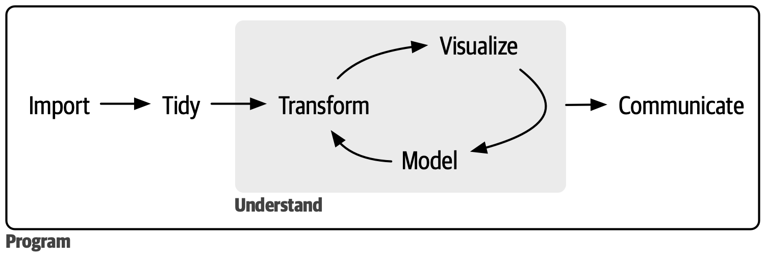
Data science is a vast field, and there’s no way you can master it all by reading a single book. This book aims to give you a solid foundation in the most important tools and enough knowledge to find the resources to learn more when necessary. Our model of the steps of a typical data science project looks something like Figure 1.

Figure 1: In our model of the data science process, you start with data import and tidying. Next, you understand your data with an iterative cycle of transforming, visualizing, and modeling. You finish the process by communicating your results to other humans.

First, you must import your data into R. This typically means that you take data stored in a file, database, or web application programming interface (API) and load it into a data frame in R. If you can’t get your data into R, you can’t do data science on it!

Once you’ve imported your data, it is a good idea to tidy it. Tidying your data means storing it in a consistent form that matches the semantics of the dataset with how it is stored. In brief, when your data is tidy, each column is a variable and each row is an observation. Tidy data is important because the consistent structure lets you focus your efforts on answering questions about the data, not fighting to get the data into the right form for different functions.

Once you have tidy data, a common next step is to transform it. Transformation includes narrowing in on observations of interest (like all people in one city or all data from the last year), creating new variables that are functions of existing variables (like computing speed from distance and time), and calculating a set of summary statistics (like counts or means). Together, tidying and transforming are called wrangling because getting your data in a form that’s natural to work with often feels like a fight!

Once you have tidy data with the variables you need, there are two main engines of knowledge generation: visualization and modeling. These have complementary strengths and weaknesses, so any real data analysis will iterate between them many times.

Visualization is a fundamentally human activity. A good visualization will show you things you did not expect or raise new questions about the data. A good visualization might also hint that you’re asking the wrong question or that you need to collect different data. Visualizations can surprise you, but they don’t scale particularly well because they require a human to interpret them.

Models are complementary tools to visualization. Once you have made your questions sufficiently precise, you can use a model to answer them. Models are fundamentally mathematical or computational tools, so they generally scale well. Even when they don’t, it’s usually cheaper to buy more computers than it is to buy more brains! But every model makes assumptions, and by its very nature, a model cannot question its own assumptions. That means a model cannot fundamentally surprise you.

The last step of data science is communication, an absolutely critical part of any data analysis project. It doesn’t matter how well your models and visualization have led you to understand the data unless you can also communicate your results to others.

Surrounding all these tools is programming. Programming is a cross-cutting tool that you use in nearly every part of a data science project. You don’t need to be an expert programmer to be a successful data scientist, but learning more about programming pays off because becoming a better programmer allows you to automate common tasks and solve new problems with greater ease.

You’ll use these tools in every data science project, but they’re not enough for most projects. There’s a rough 80/20 rule at play: you can tackle about 80% of every project using the tools you’ll learn in this book, but you’ll need other tools to tackle the remaining 20%. Throughout this book, we’ll point you to resources where you can learn more.

How this book is organized

The previous description of the tools of data science is organized roughly according to the order in which you use them in an analysis (although, of course, you’ll iterate through them multiple times). In our experience, however, learning data importing and tidying first is suboptimal because, 80% of the time, it’s routine and boring, and the other 20% of the time, it’s weird and frustrating. That’s a bad place to start learning a new subject! Instead, we’ll start with visualization and transformation of data that’s already been imported and tidied. That way, when you ingest and tidy your own data, your motivation will stay high because you know the pain is worth the effort.

Within each chapter, we try to adhere to a consistent pattern: start with some motivating examples so you can see the bigger picture, and then dive into the details. Each section of the book is paired with exercises to help you practice what you’ve learned. Although it can be tempting to skip the exercises, there’s no better way to learn than by practicing on real problems.

What you won’t learn

There are several important topics that this book doesn’t cover. We believe it’s important to stay ruthlessly focused on the essentials so you can get up and running as quickly as possible. That means this book can’t cover every important topic.

Modeling

Modeling is super important for data science, but it’s a big topic, and unfortunately, we just don’t have the space to give it the coverage it deserves here. To learn more about modeling, we highly recommend Tidy Modeling with R by our colleagues Max Kuhn and Julia Silge. This book will teach you the tidymodels family of packages, which, as you might guess from the name, share many conventions with the tidyverse packages we use in this book.

Big data

This book proudly and primarily focuses on small, in-memory datasets. This is the right place to start because you can’t tackle big data unless you have experience with small data. The tools you’ll learn throughout the majority of this book will easily handle hundreds of megabytes of data, and with a bit of care, you can typically use them to work with a few gigabytes of data. We’ll also show you how to get data out of databases and parquet files, both of which are often used to store big data. You won’t necessarily be able to work with the entire dataset, but that’s not a problem because you only need a subset or subsample to answer the question that you’re interested in.

If you’re routinely working with larger data (10–100 GB, say), we recommend learning more about data.table. We don’t teach it here because it uses a different interface than the tidyverse and requires you to learn some different conventions. However, it is incredibly faster, and the performance payoff is worth investing some time in learning it if you’re working with large data.

Python, Julia, and friends

In this book, you won’t learn anything about Python, Julia, or any other programming language useful for data science. This isn’t because we think these tools are bad. They’re not! And in practice, most data science teams use a mix of languages, often at least R and Python. But we strongly believe that it’s best to master one tool at a time, and R is a great place to start.

Prerequisites

We’ve made a few assumptions about what you already know to get the most out of this book. You should be generally numerically literate, and it’s helpful if you have some basic programming experience already. If you’ve never programmed before, you might find Hands on Programming with R by Garrett to be a valuable adjunct to this book.

You need four things to run the code in this book: R, RStudio, a collection of R packages called the tidyverse, and a handful of other packages. Packages are the fundamental units of reproducible R code. They include reusable functions, documentation that describes how to use them, and sample data.

R

To download R, go to CRAN, the comprehensive R archive network, https://cloud.r-project.org. A new major version of R comes out once a year, and there are 2-3 minor releases each year. It’s a good idea to update regularly. Upgrading can be a bit of a hassle, especially for major versions that require you to re-install all your packages, but putting it off only makes it worse. We recommend R 4.2.0 or later for this book.

RStudio

RStudio is an integrated development environment, or IDE, for R programming, which you can download from https://posit.co/download/rstudio-desktop/. RStudio is updated a couple of times a year, and it will automatically let you know when a new version is out, so there’s no need to check back. It’s a good idea to upgrade regularly to take advantage of the latest and greatest features. For this book, make sure you have at least RStudio 2022.02.0.

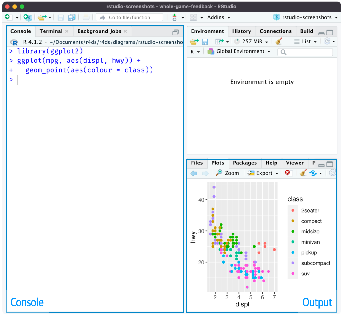
When you start RStudio, Figure 2, you’ll see two key regions in the interface: the console pane and the output pane. For now, all you need to know is that you type the R code in the console pane and press enter to run it. You’ll learn more as we go along!¹

Figure 2: The RStudio IDE has two key regions: type R code in the console pane on the left, and look for plots in the output pane on the right.

The tidyverse

You’ll also need to install some R packages. An R package is a collection of functions, data, and documentation that extends the capabilities of base R. Using packages is key to the successful use of R. The majority of the packages that you will learn in this book are part of the so-called tidyverse. All packages in the tidyverse share a common philosophy of data and R programming and are designed to work together.

You can install the complete tidyverse with a single line of code:

install.packages("tidyverse")

On your computer, type that line of code in the console, and then press enter to run it. R will download the packages from CRAN and install them on your computer.

You will not be able to use the functions, objects, or help files in a package until you load it with library(). Once you have installed a package, you can load it using the library() function:

library(tidyverse)
#> ── Attaching core tidyverse packages ───────────────────── tidyverse 2.0.0 ──
#> ✔ dplyr     1.1.4     ✔ readr     2.1.5
#> ✔ forcats   1.0.0     ✔ stringr   1.5.1
#> ✔ ggplot2   3.5.1     ✔ tibble    3.2.1
#> ✔ lubridate 1.9.3     ✔ tidyr     1.3.1
#> ✔ purrr     1.0.2     
#> ── Conflicts ─────────────────────────────────────── tidyverse_conflicts() ──
#> ✖ dplyr::filter() masks stats::filter()
#> ✖ dplyr::lag()    masks stats::lag()
#> ℹ Use the conflicted package (<http://conflicted.r-lib.org/>) to force all conflicts to become errors

This tells you that tidyverse loads nine packages: dplyr, forcats, ggplot2, lubridate, purrr, readr, stringr, tibble, tidyr. These are considered the core of the tidyverse because you’ll use them in almost every analysis.

Packages in the tidyverse change fairly frequently. You can see if updates are available by running tidyverse_update().

Other packages

There are many other excellent packages that are not part of the tidyverse because they solve problems in a different domain or are designed with a different set of underlying principles. This doesn’t make them better or worse; it just makes them different. In other words, the complement to the tidyverse is not the messyverse but many other universes of interrelated packages. As you tackle more data science projects with R, you’ll learn new packages and new ways of thinking about data.

We’ll use many packages from outside the tidyverse in this book. For example, we’ll use the following packages because they provide interesting datasets for us to work with in the process of learning R:

install.packages(
  c("arrow", "babynames", "curl", "duckdb", "gapminder", 
    "ggrepel", "ggridges", "ggthemes", "hexbin", "janitor", "Lahman", 
    "leaflet", "maps", "nycflights13", "openxlsx", "palmerpenguins", 
    "repurrrsive", "tidymodels", "writexl")
  )

We’ll also use a selection of other packages for one off examples. You don’t need to install them now, just remember that whenever you see an error like this:

library(ggrepel)
#> Error in library(ggrepel) : there is no package called ‘ggrepel’

You need to run install.packages("ggrepel") to install the package.

Running R code

The previous section showed you several examples of running R code. The code in the book looks like this:

1 + 2
#> [1] 3

If you run the same code in your local console, it will look like this:

> 1 + 2
[1] 3

There are two main differences. In your console, you type after the >, called the prompt; we don’t show the prompt in the book. In the book, the output is commented out with #>; in your console, it appears directly after your code. These two differences mean that if you’re working with an electronic version of the book, you can easily copy code out of the book and paste it into the console.

Throughout the book, we use a consistent set of conventions to refer to code:

• Functions are displayed in a code font and followed by parentheses, like sum() or mean().

• Other R objects (such as data or function arguments) are in a code font, without parentheses, like flights or x.

• Sometimes, to make it clear which package an object comes from, we’ll use the package name followed by two colons, like dplyr::mutate() or nycflights13::flights. This is also valid R code.

Acknowledgments

This book isn’t just the product of Hadley, Mine, and Garrett but is the result of many conversations (in person and online) that we’ve had with many people in the R community. We’re incredibly grateful for all the conversations we’ve had with y’all; thank you so much!

This book was written in the open, and many people contributed via pull requests. A special thanks to all 259 of you who contributed improvements via GitHub pull requests (in alphabetical order by username): @a-rosenberg, Tim Becker (@a2800276), Abinash Satapathy (@Abinashbunty), Adam Gruer (@adam-gruer), adi pradhan (@adidoit), A. s. (@Adrianzo), Aep Hidyatuloh (@aephidayatuloh), Andrea Gilardi (@agila5), Ajay Deonarine (@ajay-d), @AlanFeder, Daihe Sui (@alansuidaihe), @alberto-agudo, @AlbertRapp, @aleloi, pete (@alonzi), Alex (@ALShum), Andrew M. (@amacfarland), Andrew Landgraf (@andland), @andyhuynh92, Angela Li (@angela-li), Antti Rask (@AnttiRask), LOU Xun (@aquarhead), @ariespirgel, @august-18, Michael Henry (@aviast), Azza Ahmed (@azzaea), Steven Moran (@bambooforest), Brian G. Barkley (@BarkleyBG), Mara Averick (@batpigandme), Oluwafemi OYEDELE (@BB1464), Brent Brewington (@bbrewington), Bill Behrman (@behrman), Ben Herbertson (@benherbertson), Ben Marwick (@benmarwick), Ben Steinberg (@bensteinberg), Benjamin Yeh (@bentyeh), Betul Turkoglu (@betulturkoglu), Brandon Greenwell (@bgreenwell), Bianca Peterson (@BinxiePeterson), Birger Niklas (@BirgerNi), Brett Klamer (@bklamer), @boardtc, Christian (@c-hoh), Caddy (@caddycarine), Camille V Leonard (@camillevleonard), @canovasjm, Cedric Batailler (@cedricbatailler), Christina Wei (@christina-wei), Christian Mongeau (@chrMongeau), Cooper Morris (@coopermor), Colin Gillespie (@csgillespie), Rademeyer Vermaak (@csrvermaak), Chloe Thierstein (@cthierst), Chris Saunders (@ctsa), Abhinav Singh (@curious-abhinav), Curtis Alexander (@curtisalexander), Christian G. Warden (@cwarden), Charlotte Wickham (@cwickham), Kenny Darrell (@darrkj), David Kane (@davidkane9), David (@davidrsch), David Rubinger (@davidrubinger), David Clark (@DDClark), Derwin McGeary (@derwinmcgeary), Daniel Gromer (@dgromer), @Divider85, @djbirke, Danielle Navarro (@djnavarro), Russell Shean (@DOH-RPS1303), Zhuoer Dong (@dongzhuoer), Devin Pastoor (@dpastoor), @DSGeoff, Devarshi Thakkar (@dthakkar09), Julian During (@duju211), Dylan Cashman (@dylancashman), Dirk Eddelbuettel (@eddelbuettel), Edwin Thoen (@EdwinTh), Ahmed El-Gabbas (@elgabbas), Henry Webel (@enryH), Ercan Karadas (@ercan7), Eric Kitaif (@EricKit), Eric Watt (@ericwatt), Erik Erhardt (@erikerhardt), Etienne B. Racine (@etiennebr), Everett Robinson (@evjrob), @fellennert, Flemming Miguel (@flemmingmiguel), Floris Vanderhaeghe (@florisvdh), @funkybluehen, @gabrivera, Garrick Aden-Buie (@gadenbuie), Peter Ganong (@ganong123), Gerome Meyer (@GeroVanMi), Gleb Ebert (@gl-eb), Josh Goldberg (@GoldbergData), bahadir cankardes (@gridgrad), Gustav W Delius (@gustavdelius), Hao Chen (@hao-trivago), Harris McGehee (@harrismcgehee), @hendrikweisser, Hengni Cai (@hengnicai), Iain (@Iain-S), Ian Sealy (@iansealy), Ian Lyttle (@ijlyttle), Ivan Krukov (@ivan-krukov), Jacob Kaplan (@jacobkap), Jazz Weisman (@jazzlw), John Blischak (@jdblischak), John D. Storey (@jdstorey), Gregory Jefferis (@jefferis), Jeffrey Stevens (@JeffreyRStevens), 蒋雨蒙 (@JeldorPKU), Jennifer (Jenny) Bryan (@jennybc), Jen Ren (@jenren), Jeroen Janssens (@jeroenjanssens), @jeromecholewa, Janet Wesner (@jilmun), Jim Hester (@jimhester), JJ Chen (@jjchern), Jacek Kolacz (@jkolacz), Joanne Jang (@joannejang), @johannes4998, John Sears (@johnsears), @jonathanflint, Jon Calder (@jonmcalder), Jonathan Page (@jonpage), Jon Harmon (@jonthegeek), JooYoung Seo (@jooyoungseo), Justinas Petuchovas (@jpetuchovas), Jordan (@jrdnbradford), Jeffrey Arnold (@jrnold), Jose Roberto Ayala Solares (@jroberayalas), Joyce Robbins (@jtr13), @juandering, Julia Stewart Lowndes (@jules32), Sonja (@kaetschap), Kara Woo (@karawoo), Katrin Leinweber (@katrinleinweber), Karandeep Singh (@kdpsingh), Kevin Perese (@kevinxperese), Kevin Ferris (@kferris10), Kirill Sevastyanenko (@kirillseva), Jonathan Kitt (@KittJonathan), @koalabearski, Kirill Müller (@krlmlr), Rafał Kucharski (@kucharsky), Kevin Wright (@kwstat), Noah Landesberg (@landesbergn), Lawrence Wu (@lawwu), @lindbrook, Luke W Johnston (@lwjohnst86), Kara de la Marck (@MarckK), Kunal Marwaha (@marwahaha), Matan Hakim (@matanhakim), Matthias Liew (@MatthiasLiew), Matt Wittbrodt (@MattWittbrodt), Mauro Lepore (@maurolepore), Mark Beveridge (@mbeveridge), @mcewenkhundi, mcsnowface, PhD (@mcsnowface), Matt Herman (@mfherman), Michael Boerman (@michaelboerman), Mitsuo Shiota (@mitsuoxv), Matthew Hendrickson (@mjhendrickson), @MJMarshall, Misty Knight-Finley (@mkfin7), Mohammed Hamdy (@mmhamdy), Maxim Nazarov (@mnazarov), Maria Paula Caldas (@mpaulacaldas), Mustafa Ascha (@mustafaascha), Nelson Areal (@nareal), Nate Olson (@nate-d-olson), Nathanael (@nateaff), @nattalides, Ned Western (@NedJWestern), Nick Clark (@nickclark1000), @nickelas, Nirmal Patel (@nirmalpatel), Nischal Shrestha (@nischalshrestha), Nicholas Tierney (@njtierney), Jakub Nowosad (@Nowosad), Nick Pullen (@nstjhp), @olivier6088, Olivier Cailloux (@oliviercailloux), Robin Penfold (@p0bs), Pablo E. Garcia (@pabloedug), Paul Adamson (@padamson), Penelope Y (@penelopeysm), Peter Hurford (@peterhurford), Peter Baumgartner (@petzi53), Patrick Kennedy (@pkq), Pooya Taherkhani (@pooyataher), Y. Yu (@PursuitOfDataScience), Radu Grosu (@radugrosu), Ranae Dietzel (@Ranae), Ralph Straumann (@rastrau), Rayna M Harris (@raynamharris), @ReeceGoding, Robin Gertenbach (@rgertenbach), Jajo (@RIngyao), Riva Quiroga (@rivaquiroga), Richard Knight (@RJHKnight), Richard Zijdeman (@rlzijdeman), @robertchu03, Robin Kohrs (@RobinKohrs), Robin (@Robinlovelace), Emily Robinson (@robinsones), Rob Tenorio (@robtenorio), Rod Mazloomi (@RodAli), Rohan Alexander (@RohanAlexander), Romero Morais (@RomeroBarata), Albert Y. Kim (@rudeboybert), Saghir (@saghirb), Hojjat Salmasian (@salmasian), Jonas (@sauercrowd), Vebash Naidoo (@sciencificity), Seamus McKinsey (@seamus-mckinsey), @seanpwilliams, Luke Smith (@seasmith), Matthew Sedaghatfar (@sedaghatfar), Sebastian Kraus (@sekR4), Sam Firke (@sfirke), Shannon Ellis (@ShanEllis), @shoili, Christian Heinrich (@Shurakai), S’busiso Mkhondwane (@sibusiso16), SM Raiyyan (@sm-raiyyan), Jakob Krigovsky (@sonicdoe), Stephan Koenig (@stephan-koenig), Stephen Balogun (@stephenbalogun), Steven M. Mortimer (@StevenMMortimer), Stéphane Guillou (@stragu), Sulgi Kim (@sulgik), Sergiusz Bleja (@svenski), Tal Galili (@talgalili), Alec Fisher (@Taurenamo), Todd Gerarden (@tgerarden), Tom Godfrey (@thomasggodfrey), Tim Broderick (@timbroderick), Tim Waterhouse (@timwaterhouse), TJ Mahr (@tjmahr), Thomas Klebel (@tklebel), Tom Prior (@tomjamesprior), Terence Teo (@tteo), @twgardner2, Ulrik Lyngs (@ulyngs), Shinya Uryu (@uribo), Martin Van der Linden (@vanderlindenma), Walter Somerville (@waltersom), @werkstattcodes, Will Beasley (@wibeasley), Yihui Xie (@yihui), Yiming (Paul) Li (@yimingli), @yingxingwu, Hiroaki Yutani (@yutannihilation), Yu Yu Aung (@yuyu-aung), Zach Bogart (@zachbogart), @zeal626, Zeki Akyol (@zekiakyol).

Colophon

An online version of this book is available at https://r4ds.hadley.nz. It will continue to evolve in between reprints of the physical book. The source of the book is available at https://github.com/hadley/r4ds. The book is powered by Quarto, which makes it easy to write books that combine text and executable code.

---

1. If you’d like a comprehensive overview of all of RStudio’s features, see the RStudio User Guide at https://docs.posit.co/ide/user.